
Base Guide 7.2
Chapter 5
Queries
This document is Copyright © 2021 by the LibreOffice Documentation Team. Contributors are listed below. You may distribute it and/or modify it under the terms of either the GNU General Public License (https://www.gnu.org/licenses/gpl.html), version 3 or later, or the Creative Commons Attribution License (https://creativecommons.org/licenses/by/4.0/), version 4.0 or later.
All trademarks within this guide belong to their legitimate owners.
|
Pulkit Krishna |
Dan Lewis |
|
|
Robert Großkopf |
Pulkit Krishna |
Jost Lange |
|
Dan Lewis |
Hazel Russman |
Jochen Schiffers |
|
Steve Schwettman |
Jean Hollis Weber |
|
Please direct any comments or suggestions about this document to the Documentation Team’s mailing list: documentation@global.libreoffice.org.
Note
Everything you send to a mailing list, including your email address and any other personal information that is written in the message, is publicly archived and cannot be deleted.
Published December 2021. Based on LibreOffice 7.2 Community.
Other versions of LibreOffice may differ in appearance and functionality.
Queries to a database are the most powerful tool that we have to use databases in a practical way. They can bring together data from different tables, calculate results where necessary, and quickly filter a specific record from a mass of data. The large Internet databases that people use every day exist mainly to deliver a quick and practical result for the user from a huge amount of information by thoughtful selection of keywords – including the search-related advertisements that encourage people to make purchases.
Queries can be entered both in the GUI and directly as SQL code. In both cases a window opens, where you can create a query and also correct it if necessary.
The creation of queries using the Wizard is briefly described in Chapter 8 of the Getting Started Guide, Getting Started with Base. Here we shall explain the direct creation of queries in Design View.
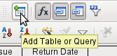
In the main database window, click the Queries icon in the Databases section, then in the Tasks section, click Create Query in Design View. Two dialogs appear. One provides the basis for a design-view creation of the query; the other serves to add tables, views, or queries to the current query.
As our simple form refers to the Loan table, we will first explain the creation of a query using this table.
From the tables available, select the Loan table. This window allows multiple tables (and also views and queries) to be combined. To select a table, click its name and then click the Add button. Or, double-click the table’s name. Either method adds the table to the graphical area of the Query Design dialog (Figure 1).
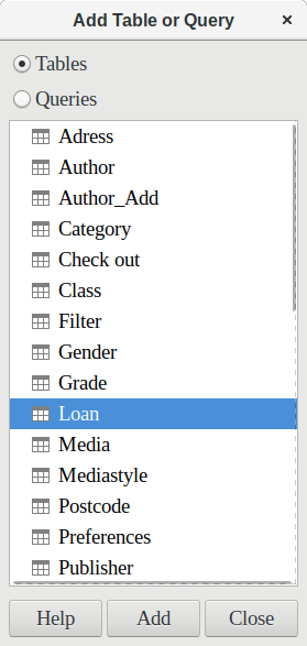
When all necessary tables have been selected, click the Close button. Additional tables and queries can be added later if required. However, no query can be created without at least one table, so a selection must be made at the beginning.
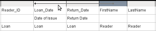
Figure 1: Areas of the Query Design dialog
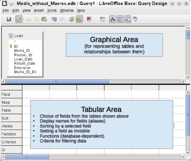
Figure 1 shows the basic divisions of the Query Design dialog: the graphical area displays the tables that are to be linked to the query. Their relationships to each other in relation to the query may also be shown. The tabular area is for the selection of fields for display, or for setting conditions related to these fields.
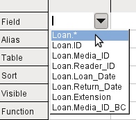
Click on the field in the first column in the tabular area to reveal a down arrow. Click this arrow to open the drop-down list of available fields. The format is Table_name.Field_name – which is why all field names here begin with the word Loan.
The selected field designation Loan.* has a special meaning. Here one click allows you to add all fields from the underlying table to the query. When you use this field designation with the wildcard * for all fields, the query becomes indistinguishable from the table.
Tip
For a quick transfer of all the fields in a table into a query, just click the table view in the graphical interface (Loan.* above).
A double-click on a field inserts that field into the tabular area at the next free position.
The first five fields of the Loan table are selected. Queries in Design Mode can always be run as tests. This causes a tabular view of the data to appear above the graphical view of the Loan table with its list of fields. A test run of a query is always useful before saving it, to clarify whether the query actually achieves its goal. Often a logical error prevents a query from retrieving any data at all. In other cases it can happen that precisely those records are displayed that you wished to exclude.
In principle a query that produces an error message in the underlying database cannot be saved until the error is corrected.
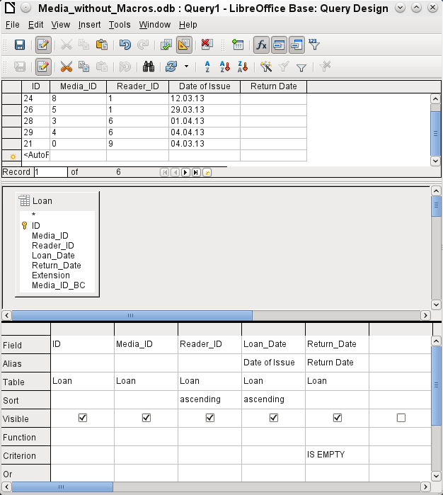
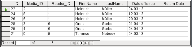
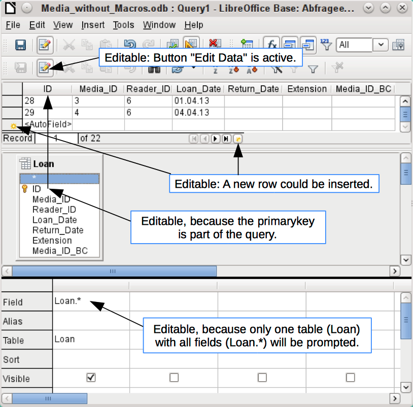
Figure 2: An editable query
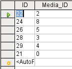
Figure 3: A non-editable query
In the above test, pay special attention to the first column of the query result. The active record marker (green arrow) always appears on the left side of the table, here pointing to the first record as the active record. While the first field of the first record in Figure 2 is highlighted, the corresponding field in Figure 3 shows only a dashed border. The highlight indicates that this field can be modified. The records, in other words, are editable. The dashed border indicates that this field cannot be modified. Figure 2 also contains an extra line for the entry of a new record, with the ID field already marked as <AutoField>. This also shows that new entries are possible.
Tip
A basic rule is that no new entries are possible if the primary key in the queried table is not included in the query.
The Loan_Date and Return_Date fields are given aliases. This does not cause them to be renamed but only to appear under these names for the user of the query.
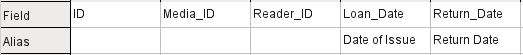
The table view above shows how the aliases replace the actual field names.

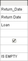
The Return_Date field is given not just an alias but also a search criterion, which will cause only those records to be displayed for which the Return_Date field is empty. (Enter IS EMPTY in the Criterion row of the Return_Date field.) This exclusion criterion will cause only those records to be displayed that relate to media that have not yet been returned.
To learn the SQL language better, it is worth switching from time to time between Design Mode and SQL Mode.
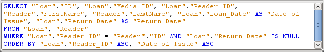
Here the SQL formula created by our previous choices is revealed. To make it easier to read, some line breaks have been included. Unfortunately the editor does not store these line breaks, so when the query is called up again, it will appear as a single continuous line breaking at the window edge.
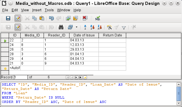
SELECT begins the selection criteria. AS specifies the field aliases to be used. FROM shows the table which is to be used as the source of the query. WHERE gives the conditions for the query, namely that the Return_Date field is to be empty (IS NULL). ORDER BY defines the sort criteria, namely ascending order (ASC – ascending) for the two fields Reader_ID and Loan_Date. This sort specification illustrates how the alias for the Loan_Date field can be used within the query itself.
Tip
When working in Design View Mode, use IS EMPTY to require a field be empty. When working in SQL Mode, use IS NULL which is what SQL (Structured Query Language) requires.
When you want to sort by descending order using SQL, use DESC instead of ASC.
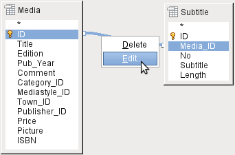
So far the Media_ID and Reader_ID fields are only visible as numeric fields. The readers’ names are unclear. To show these in a query, the Reader table must be included. For this purpose we return to Design Mode. Then a new table can be added to the Design view.
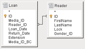
Here further tables or queries can subsequently be added and made visible in the graphical user interface. If links between the tables were declared at the time of their creation (see Chapter 3, Tables), then these tables are shown with the corresponding direct links.
If a link is absent, it can be created at this point by dragging the mouse from "Loan"."Reader_ID" to "Reader"."ID".
Note
Linking tables only works at the moment in the internal database or in external relational databases. For example, tables from a spreadsheet cannot be linked together. They must first be imported into an internal database.
To create a link between the tables, a simple import is sufficient without additional creation of a primary key.
Now fields from the Reader table can be entered into the tabular area. The fields are initially added to the end of the query.
The position of the fields can be corrected in the tabular area of the editor using the mouse. So for example, the FirstName field has been dragged into position directly before the Loan_Date field.
Now the names are visible. The Reader_ID has become superfluous. Also sorting by LastName and FirstName makes more sense than sorting by Reader_ID.
This query is no longer suitable for use as a query that allows new entries into the resulting table, since it lacks the primary key for the added Reader table. Only if this primary key is built in, does the query become editable again. In fact it then becomes completely editable so that the readers’ names can also be altered. For this reason, making query results editable is a facility that should be used with extreme caution, if necessary under the control of a form.
Caution
Having a query that you can edit can create problems. Editing data in the query also edits data in the underlying table and the records contained in the table. The data may not have the same meaning. For example, change the name of the reader, and you have also changed what books the reader has borrowed and returned.
If you have to edit data, do so in a form so you can see the effects of editing data.
Even when a query can be further edited, it is not so easy to use as a form with list boxes, which show the readers’ names but contain the Reader_ID from the table. List boxes cannot be added to a query; they are only usable in forms.
If we now switch back to SQL View, we see that all fields are now shown in double quotes: "Table _name"."Field_name". This is necessary so that the database knows from which table the previously selected fields come from. After all, fields in different tables can easily have the same field names. In the above table structure this is particularly true of the ID field.
Note
The following query works without putting table names in front of the field names:
SELECT "ID", "Number", "Price" FROM "Stock", "Dispatch" WHERE "Dispatch"."stockID" = "Stock"."ID"
Here the ID is taken from the table which comes first in the FROM definition. The table definition in the WHERE Formula is also superfluous, because stockID only occurs once (in the Dispatch table) and ID was clearly taken from the Stock table (from the position of the table in the query).
If a field in the query has an alias, it can be referred to – for example in sorting – by this alias without a table name being given. Sorting is carried out in the graphical user interface according to the sequence of fields in the tabular view. If instead you want to sort first by "Loan_Date" and then by "Loan"."Reader_ID", that can be done if:
The sequence of fields in the table area of the graphical user interface is changed (drag and drop "Loan_Date" to the left of "Loan"."Reader_ID", or
An additional field is added, set to be invisible, just for sorting (however, the editor will register this only temporarily if no alias was defined for it) [add another "Loan_Date" field just before "Loan"."Reader_ID" or add another "Loan"."Reader_ID" field just after "Loan_Date"], or
The text for the ORDER BY command in the SQL editor is altered correspondingly (ORDER BY "Loan_Date", "Loan"."Reader_ID").
Tip
A query may require a field that is not part of the query output. In the graphic in the next section, Return_Date is an example. This query is searching for records that do not contain a return date. This field provides a criterion for the query but no useful visible data.
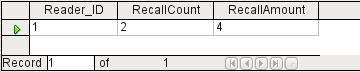
The use of functions allows a query to provide more than just a filtered view of the data in one or more tables. The following query calculates how many media have been loaned out, depending on the Reader_ID.
For the ID of the Loan table, the Count function is selected. In principle it makes no difference which field of a table is chosen for this. The only condition is: The field must not be empty in any of the records. For this reason, the primary key field, which is never empty, is the most suitable choice. All fields with a content other than NULL are counted.
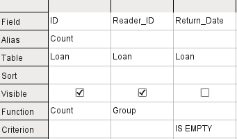
For the Reader_ID, which gives access to reader information, the Grouping function is chosen. In this way, the records with the same Reader_ID are grouped together. The result shows the number of records for each Reader_ID.
As a search criterion, the Return_Date is set to "IS EMPTY", as in the previous example. (Below, the SQL for this is WHERE "Return_Date" IS NULL.)
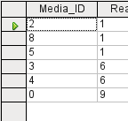
The result of the query shows that Reader_ID '0' has a total of 3 media on loan. If the Count function had been assigned to the Return_Date instead of the ID, every Reader_ID would have '0' media on loan, since Return_date is predefined as NULL.
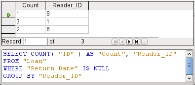
The corresponding formula in SQL code is shown above.
Altogether the graphical user interface provides the functions shown to the right, which correspond to functions in the underlying HSQLDB.
For an explanation of the functions, see “Query enhancement using SQL Mode” on page 1.
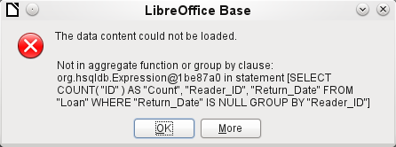
If one field in a query is associated with a function, all the remaining fields mentioned in the query must also be associated with functions if they are to be displayed. If this is not ensured, you get the following error message:
A somewhat free translation would be: The following expression contains no aggregate function or grouping.
Tip
When using Design View Mode, a field is only visible if the Visible row contains a check mark for the field. When using SQL Mode, a field is only visible when it follows the keyword SELECT.
Note
When a field is not associated with a function, the number of rows in the query output is determined by the search conditions. When a field is associated with a function, the number of rows in the query output is determined by whether there is any grouping or not. If there is no grouping, there is only one row in the query output. If there is grouping, the number of rows matches the number of distinct values that the grouping field has. So, all of the visible fields must either be associated with a function or be associated with a grouping statement to prevent this conflict in the query output.
After this, the complete query is listed in the error message, but unfortunately without the offending field being named specifically. In this case the field Return_Date has been added as a displayed field. This field has no function associated with it and is not included in the grouping statement either.
The information provided by using the More button is not very illuminating for the normal database user. It just displays the SQL error code.
To correct the error, remove the check mark in the Visible row for the Return_Date field. Its search condition (Criterion) is applied when the query is run, but it is not visible in the query output.
Using the GUI, basic calculations and additional functions can be used.
Suppose that a library does not issue recall notices when an item is due for return, but issues overdue notices in cases where the loan period has expired and the item has not been returned. This is common practice in school and public libraries that issue loans only for short, fixed periods. In this case the issue of an overdue notice automatically means that a fine must be paid. How do we calculate these fines?
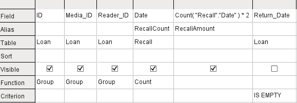
In the query shown above, the Loan and Recalls tables are queried jointly. From the count of the data entries in the table Recalls, the total number of recall notices is determined. The fine for overdue media is set in the query to $2.00. Instead of a field name, the field designation is given as Count(Recalls.Date)*2. The graphical user interface adds the quotation marks and converts the term “count” into the appropriate SQL command.
Caution
Only for people who use a comma for their decimal separator:
If you wish to enter numbers with decimal places using the GUI, you must ensure that a decimal point rather than a comma is used as a decimal separator within the final SQL statement. Commas are used as field separators, so new query fields are created for the decimal part.
An entry with a comma in the SQL view always leads to a further field containing the numerical value of the decimal part.
The query now yields for each medium still on loan the fines that have accrued, based on the recall notices issued and the additional multiplication field. The following query structure will also be useful for calculating the fines due from individual users.
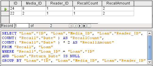
The "Loan"."ID" and "Loan"."Media_ID" fields have been removed. They were used in the previous query to create by grouping a separate record for each medium. Now we will be grouping only by the reader. The result of the query looks like this:

Instead of listing the media for Reader_ID = 0 separately, all the "Recalls"."Date" fields have been counted and the total of $8.00 entered as the fine due.
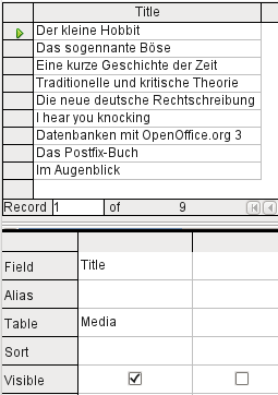
When data is searched for in tables or forms, the search is usually limited to one table or one form. Even the path from a main form to a subform is not navigable by the built-in search function. For such purposes, the data to be searched for are better collected by using a query.
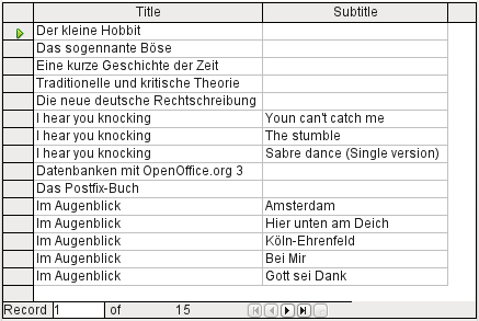
The simple query for the Title field from the Media table shows the test entries for this table, 9 records in all. But if you enter Subtitle into the query table, the record content of the Media table is reduced to only 2 Titles. Only for these two Titles are there also Subtitles in the table. For all the other Titles, no subtitles exist. This corresponds to the join condition that only those records for which the Media_ID field in the Subtitle table is equal to the ID field in the Media table should be shown. All other records are excluded.
The join conditions must be opened for editing to display all the desired records. We refer here not to joins between tables in Relationship design but to joins within queries.
By default, relationships are set as Inner Joins. The window provides information on the way this type of join works in practice.
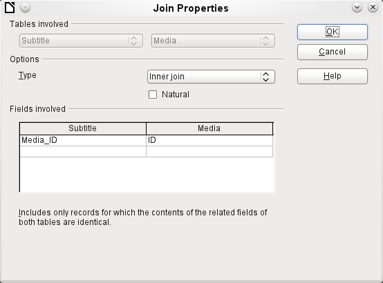
The two previously selected tables are listed as Tables Involved. They are not selectable here. The relevant fields from the two tables are read from the table definitions. If there is no relationship specified in the table definition, one can be created at this point for the query. However, if you have planned your database in an orderly manner using HSQLDB, there should be no need to alter these fields.
The most important setting is the Join option. Here relationships can be so chosen that all records from the Subtitle table are selected, but only those records from Media which have a subtitle entered in the Subtitle table.
Or you can choose the opposite: that in any case all records from the Media table are displayed, regardless of whether they have a subtitle.
The Natural option specifies that the linked fields in the tables are treated as equal. You can also avoid having to use this setting by defining your relationships properly at the very start of planning your database.
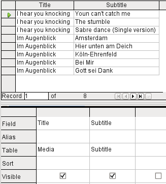
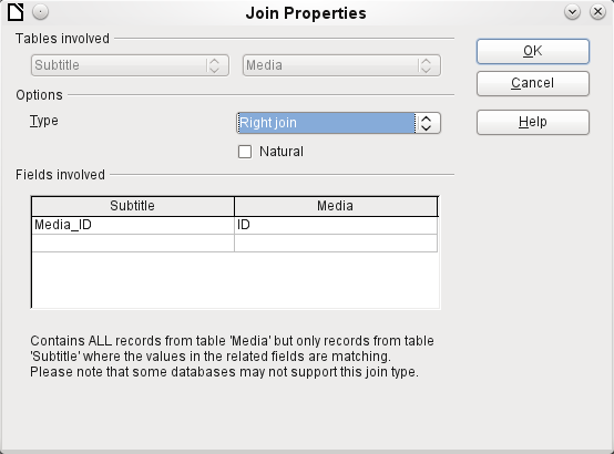
For the type Right join, the description shows that all records from the Media table will be displayed (Subtitle RIGHT JOIN Media). As there is no Subtitle that lacks a title in Media but there are certainly Titles in Media that lack a Subtitle, this is the right choice.
After confirming the Right join, the query results look as we wanted them. Title and Subtitle are displayed together in one query. Naturally Titles appear more than once as with the previous relationship. However as long as hits are not being counted, this query can be used further as a basis for a search function. See the code fragments in this chapter, in Chapter 8, Database Tasks, and in Chapter 9, Macros.
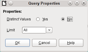
Starting with version 4.1 of LibreOffice, it is possible to define additional properties in the query editor.
Figure 4: Opening query properties in the query editor
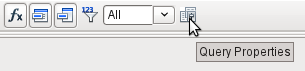
Next to the button for opening the Query Properties is a combo box for regulating the number of displayed records as well as a button for Distinct Values. These functions are repeated in the following dialog:
The Distinct Values setting determines whether the query should suppress duplicate records.
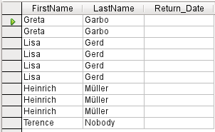
Suppose a query is made to determine which readers still have items out on loan. Their names are displayed if the return date field is empty. The names are displayed more than once for readers who have multiple items on loan.
If you choose Distinct Values, records with the same content disappear.
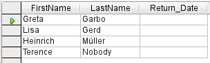
The query then looks like this:
The original query:
SELECT "Reader"."FirstName", "Reader"."LastName" …
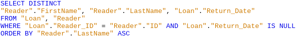
Adding DISTINCT to the query suppresses the duplicate records.
SELECT DISTINCT "Reader"."FirstName", "Reader"."LastName" …
The ability to specify unique records was also present in earlier versions. However it was necessary to switch from design view to SQL view to insert the DISTINCT qualifier. This property is therefore backward-compatible with previous versions of LO without causing any problems.
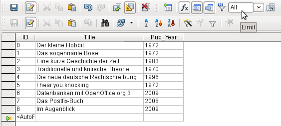
The Limit setting determines how many records are to be displayed in the query. Only a limited number of records are reproduced.
All records in the Media table are displayed. The query is editable as it includes the primary key.
Only the first five records are displayed (ID 0-4). A sort was not requested, so the default sort order by primary key is used. Despite the limitation in output, the query can be further edited. This distinguishes input in the graphical interface from what, in previous versions, was only accessible using SQL.
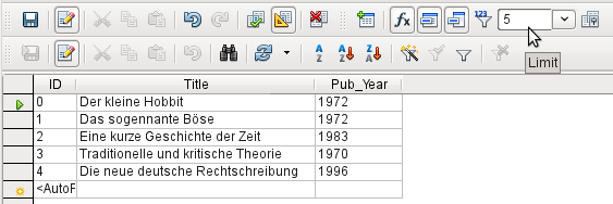
The original query has simply had “LIMIT 5” added. The size of the limit can be whatever you need.

Caution
Setting limits in the graphical interface is not backward-compatible. In all LO versions before 4.1, a limit could only be set in direct SQL mode. The limit then required a sort (ORDER BY …) or a condition (WHERE …).
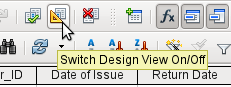
If during graphical entry you use View > Switch Design View On/Off to switch Design View off, you see the SQL command for what previously appeared in Design View. This is the best way for beginners to learn the Standard Query Language for Databases. Sometimes it is also the only way to enter a query into the database when the GUI cannot translate your requirements into the necessary SQL commands.
SELECT * FROM "Table_name"
This will show everything that is in the Table_name table. The "*" represents all the fields of the table.
SELECT * FROM "Table_name" WHERE "Field_name" = 'Karl'
Here there is a significant restriction. Only those records are displayed for which the field Field_name contains the term ‘Karl’ – the exact term, not for example ‘Karl Egon’.
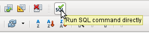
Sometimes queries in Base cannot be carried out using the GUI, as particular commands may not be recognized. In such cases it is necessary to switch Design View off and use Edit > Run SQL command directly for direct access to the database. This method has the disadvantage that you can only work with the query in SQL Mode.
Direct use of SQL commands is also accessible using the graphical user interface, as the above figure shows. Click the icon highlighted (Run SQL command directly) to turn the Design View Off/On icon off. Now when you click the Run icon, the query runs the SQL commands directly.
Here is an example of the extensive possibilities available for posing questions to the database and specifying the type of result required:
SELECT [{LIMIT <offset> <limit> | TOP <limit>}][ALL | DISTINCT]
{ <Select-Formulation> | "Table_name".* | * } [, ...]
[INTO [CACHED | TEMP | TEXT] "new_Table"]
FROM "Table_list"
[WHERE SQL-Expression]
[GROUP BY SQL-Expression [, ...]]
[HAVING SQL-Expression]
[{ UNION [ALL | DISTINCT] | {MINUS [DISTINCT] | EXCEPT [DISTINCT] } |
INTERSECT [DISTINCT] } Query statement]
[ORDER BY Order-Expression [, ...]]
[LIMIT <limit> [OFFSET <offset>]];
[{LIMIT <offset> <limit> | TOP <limit>}]:
[ALL | DISTINCT]
<Select-Formulation>
{ Expression | COUNT(*) |
{ COUNT | MIN | MAX | SUM | AVG | SOME | EVERY | VAR_POP | VAR_SAMP | STDDEV_POP | STDDEV_SAMP }
([ALL | DISTINCT]] Expression) } [[AS] "display_name"]
Note
Calculations within a database sometimes lead to unexpected results. Suppose a database contains the grades awarded for some classwork and you wish to calculate the average grade.
First you must add up all the grades. Suppose the sum is 80. Now this must be divided by the number of pupils (say 30). The query yields 2.
This occurs because you are working with fields of type INTEGER. The calculation must therefore yield an integer value. You need to have at least one value of the type DECIMAL in your calculation. You can achieve this either by using a HSQLDB conversion function or (more simply) you can divide by 30.0 rather than 30. This will give a result with one decimal place. Dividing by 30.00 gives two decimal places. Be careful to use English-style decimal points. The use of commas in queries is reserved for field separators.
COUNT | MIN | MAX | SUM | AVG | SOME | EVERY | VAR_POP | VAR_SAMP | STDDEV_POP | STDDEV_SAMP
Tip
This function also fails on time fields. Here the following may be useful:
SELECT (SUM( HOUR("Time") )*3600 + SUM( MINUTE("Time") ))*60 + SUM( SECOND("Time") ) AS "seconds" FROM "Table"
The sum displayed is made up of separate hours, minutes and seconds. Then it is modified to yield the overall total in a single unit, in this case seconds. Here then only integers are added by the sum function. Now if you use:
SELECT ((SUM( HOUR("Time") )*3600 + SUM( MINUTE("Time") ))*60 + SUM( SECOND("Time") )) / 3600.0000 AS "hours" FROM "Table"
you will get a time in hours with the minutes and seconds as decimal places. With suitable formatting, you can turn this back to a normal time value in a query or form.
Tip
The Boolean field type is Yes/No[BOOLEAN]. However, this field contains only 0 or 1. In query search conditions, use either TRUE, 1, FALSE or 0. For the Yes condition, you can use either TRUE or 1. For the No condition, use either FALSE or 0. If you try to use either “Yes” or “No” instead, you get an error message. Then you will have to correct your error.
SELECT "Class", EVERY("Swimmer")
FROM "Table1"
GROUP BY "Class";
"Table_name".* | * [, ...]
[INTO [CACHED | TEMP | TEXT] "new_table"]
FROM <Table_list>
"Table_name 1" [{CROSS | INNER | LEFT OUTER | RIGHT OUTER} JOIN "Table_name 2" ON Expression] [, ...]
SELECT "Table1"."Name", "Table2"."Class"
FROM "Table1", "Table2"
WHERE "Table1"."ClassID" = "Table2"."ID"
SELECT "Table1"."Name", "Table2"."Class"
FROM "Table1"
JOIN "Table2"
ON "Table1"."ClassID" = "Table2"."ID"
SELECT "Table1"."Name", "Table2"."Class"
FROM "Table1"
LEFT JOIN "Table2"
ON "Table1"."ClassID" = "Table2"."ID"
SELECT "Table1"."Player1", "Table2"."Player2"
FROM "Table1" AS "Table1"
CROSS JOIN "Table2" AS "Table1"
WHERE "Table1"."Player1" <> "Table2"."Player2"
SELECT "Table1"."Name", "Table2"."Class"
FROM "Table1"
JOIN "Table2"
ON "Table1"."ClassID" = "Table2"."ID"
SELECT "Table1"."Name", "Table2"."Class"
FROM "Table1" AS "Table1"
CROSS JOIN "Table2" AS "Table2"
WHERE "Table1"."ClassID" = "Table2"."ID"
[WHERE SQL-Expression]
[GROUP BY SQL-Expression [, …]]
SELECT "Name", SUM("Input"-"Output") AS "Balance"
FROM "Table1"
GROUP BY "Name";
Tip
When fields are processed using a particular function (for example COUNT, SUM …), all fields that are not processed with a function but should be displayed are grouped together using GROUP BY.
[HAVING SQL-Expression]
SELECT "Name", "Runtime"
FROM "Table1"
GROUP BY "Name", "Runtime"
HAVING MIN("Runtime") < '00:40:00';
SELECT "Name", SUM("Input"-"Output") AS "Balance"
FROM "Table1"
GROUP BY "Name"
HAVING SUM("Input"-"Output") > 0;
[SQL Expression]
[NOT] condition [{ OR | AND } condition]
SELECT *
FROM "Table_name"
WHERE NOT "Return_date" IS NULL AND "ReaderID" = 2;
SELECT *
FROM "Table_name"
WHERE NOT ("Return_date" IS NULL AND "ReaderID" = 2);
[SQL Expression]: conditions
{ value [|| value]
SELECT "Surname" || ', ' || "First_name" AS "Name"
FROM "Table_name"
| value { = | < | <= | > | >= | <> |!= } value
| value IS [NOT] NULL
| EXISTS(Query_result)
SELECT "Name"
FROM "Table1"
WHERE EXISTS
(SELECT "First_name"
FROM "Table2"
WHERE "Table2"."First_name" = "Table1"."Name")
| Value BETWEEN Value AND Value
SELECT "Name"
FROM "Table_name"
WHERE "Name" BETWEEN 'A' AND 'E';
| value [NOT] IN ( {value [, ...] | Query result } )
| value [NOT] LIKE value [ESCAPE] value }
SELECT "Name"
FROM "Table_name"
WHERE "Name" LIKE '\_%' ESCAPE '\'
[SQL Expression]: values
[+ | -] { Expression [{ + | - | * | / | || } Expression]
SELECT "Surname"||', '||"First_name"
FROM "Table"
| ( Condition )
| Function ( [Parameter] [,...] )
| Query result which yields exactly one answer
| {ANY|ALL} (Queryresult which yields exactly one answer from a whole column)
[SQL Expression]: Expression
{ 'Text' | Integer | Floating-point number
| ["Table".]"Field" | TRUE | FALSE | NULL }
UNION [ALL | DISTINCT] Query_result
SELECT "First_name"
FROM "Table1"
UNION DISTINCT
SELECT "First_name"
FROM "Table2";
SELECT
"Sales_price"
FROM "Stock" WHERE "Stock_ID" = 1
UNION
SELECT
"Rebate_price_1"
FROM "Stock" WHERE "Stock_ID" = 1
UNION
SELECT
"Rebate_price_2"
FROM "Stock" WHERE "Stock_ID" = 1;
MINUS [DISTINCT] | EXCEPT [DISTINCT] Query_result
SELECT "First_name"
FROM "Table1"
EXCEPT
SELECT "First_name"
FROM "Table2";
INTERSECT [DISTINCT] Query_result
SELECT "First_name"
FROM "Table1"
INTERSECT
SELECT "First_name"
FROM "Table2";
[ORDER BY Ordering-Expression [, …]]
SELECT "First_name", "Surname" AS "Name"
FROM "Table1"
ORDER BY "Surname";
SELECT "First_name", "Surname" AS "Name"
FROM "Table1"
ORDER BY 2;
SELECT "First_name", "Surname" AS "Name"
FROM "Table1"
ORDER BY "Name";
Queries can reproduce fields with changed names.
SELECT "First_name", "Surname" AS "Name"
FROM "Table1"
The Surname field is called Name in the display.
If a query involves two tables, each field name must be preceded by the name of the table:
SELECT "Table1"."First_name", "Table1"."Surname" AS "Name", "Table2"."Class"
FROM "Table1", "Table2"
WHERE "Table1"."Class_ID" = "Table2"."ID"
The table name can also be given an alias, but this will not be reproduced in table view. If such an alias is set, all the table names in the query must be altered accordingly:
SELECT "a"."First_name", "a"."Surname" AS "Name", "b"."Class"
FROM "Table1" AS "a", "Table2" AS "b"
WHERE "a"."Class_ID" = "b"."ID"
The assignment of an alias for a table can be carried out more briefly without using the term AS:
SELECT "a"."First_name", "a"."Surname" "Name", "b"."Class"
FROM "Table1" "a", "Table2" "b"
WHERE "a"."Class_ID" = "b"."ID"
This however makes the code less readable. Because of this, the abbreviated form should be used only in exceptional circumstances.
Note
Unfortunately the code for the query editor in the graphical user interface has recently been changed so that alias designations are created without using the prefix AS. This is because, when external databases are used, whose method of specifying aliases cannot be predicted, the inclusion of AS has led to error messages.
If the query code is opened for editing, not directly in SQL but using the GUI, existing aliases lose their AS prefix. If this is important to you, you must always edit queries in SQL view.
An alias name also makes it possible to use a table with corresponding filtering more than once within a query:
SELECT "KasseAccount"."Balance", "Account"."Date",
"a"."Balance" AS "Actual",
"b"."Balance" AS "Desired"
FROM "Account"
LEFT JOIN "Account" AS "a"
ON "Account"."ID" = "a"."ID" AND "a"."Balance" >= 0
LEFT JOIN "Account" AS "b"
ON "Account"."ID" = "b"."ID" AND "b"."Balance" < 0
List box fields show a value that does not correspond to the content of the underlying table. They are used to display the value assigned by a user to a foreign key rather than the key itself. The value that is finally saved in the form must not occur in the first position of the list box field.
SELECT "FirstName", "ID"
FROM "Table1";
This query would show all first names and the primary key "ID" values that the form’s underlying table provides. Of course it is not yet optimal. The first names appear unsorted and, in the case of identical first names, it is impossible to determine which person is intended.
SELECT "FirstName"||' '||"LastName", "ID"
FROM "Table1"
ORDER BY "FirstName"||' '||"LastName";
Now the first name and the surname both appear, separated by a space. The names become distinguishable and are also sorted. But the sort follows the usual logic of starting with the first letter of the string, so it sorts by first name and only then by surname. A different sort order to that in which the fields are displayed would only be confusing.
SELECT "LastName"||', '||"FirstName", "ID"
FROM "Table1"
ORDER BY "LastName"||', '||"FirstName";
This now leads to a sorting that corresponds better to normal custom. Family members appear together, one under another; however different families with the same surname would be interleaved. To distinguish them, we would need to group them differently within the table.
There is one final problem: if two people have the same surname and first name, they will still not be distinguishable. One solution might be to use a name suffix. But imagine how it would look if a salutation read Mr "Müller II"!
SELECT "LastName"||', '||"FirstName"||' - ID:'||"ID", "ID"
FROM "Table1"
ORDER BY "LastName"||', '||"FirstName"||"ID";
Here all records are distinguishable. What is actually displayed is "LastName, FirstName – ID:ID value".
In the loan form, there is a list box which only shows the media that have not yet been loaned out. It is created using the following SQL formula:
SELECT "Title" || ' - Nr. ' || "ID", "ID"
FROM "Media"
WHERE "ID" NOT IN
(SELECT "Media_ID"
FROM "Loan"
WHERE "Return_Date" IS NULL)
ORDER BY "Title" || ' - Nr. ' || "ID" ASC
It is important that this list field is always be updated if a medium within it goes out on loan.
The following list field shows the content of several fields in tabular form so that elements that belong together are directly under one another.
To make such a representation work, you must first choose a suitable fixed-width font. Courier or any mono-font such as Liberation Mono could be used here. You create the tabular form using SQL code:
SELECT
LEFT("Stock"||SPACE(25),25) || ' - ' ||
RIGHT(SPACE(8)||"Price",8) || ' €',
"ID"
FROM "Stock"
ORDER BY ("Stock" || ' - ' || "Price" || ' $') ASC
The content of the Stock field has been padded with spaces so that the whole string has a minimum length of 25 characters. Afterwards the first 25 letters are placed there and the surplus cut.
It gets more complicated when the contents of the listfield contains non-printing characters like newlines. Then the code must be customized to fit:
SELECT
LEFT(REPLACE("Stock",CHAR(10),' ')||SPACE(25), 25) || ' - ' || ...
This replaces a newline in Linux with a space. In Windows you must additionally remove the carriage return (CHAR(13)).
The number of spaces that are necessary can also be determined on a per-query basis. This prevents a value of “Stock” being accidentally truncated.
SELECT
LEFT("Stock"||SPACE((SELECT MAX(LENGTH("Stock")) FROM "Stock")), (SELECT MAX(LENGTH("Stock")) FROM "Stock"))|| ' - ' ||
RIGHT(' '||"Price",8) || ' €',
"ID"
FROM "Stock"
ORDER BY ("Stock" || ' - ' || "Price" || ' $') ASC
As the price is to be shown right-justified, it is left-padded with spaces and placed a maximum of eight characters from the right. The representation selected will work for all prices up to $ 99999,99.
If you want to replace the decimal point with a comma within SQL, you will need some extra code:
REPLACE(RIGHT(' '||"Price",8),'.',',')
If you wish a form to display additional Information that would otherwise not be visible, there are various query possibilities. The simplest is to retrieve this information with independent queries and insert the results into the form. The disadvantage of this method is that changes in the records may affect the query result, but unfortunately these changes are not automatically displayed.
Here is an example from the sphere of stock control for a simple checkout.
The checkout table contains totals and foreign keys for stock items, and a receipt number. The shopper has very little information if there is no additional query result printed on the receipt. After all, the items are identified only by reading in a barcode. Without a query, the form shows only:
|
Total |
Barcode |
|
3 |
17 |
|
2 |
24 |
What is hidden behind the numbers cannot be made visible by using a list box, as the foreign key is input directly using the barcode. In the same way, it is impossible to use a list box next to the item to show at least the unit price.
Here a query can help.
SELECT "Checkout"."Receipt_ID", "Checkout"."Total", "Stock"."Item", "Stock"."Unit_Price", "Checkout"."Total"*"Stock"."Unit_price" AS "Total_Price"
FROM "Checkout", "Item"
WHERE "Stock"."ID" = "Checkout"."Item_ID";
Now at least after the information has been entered, we know how much needs to be paid for 3 * Item'17'. In addition only the information relevant to the corresponding Receipt_ID needs to be filtered through the form. What is still lacking is what the customer needs to pay overall.
SELECT "Checkout"."Receipt_ID", SUM("Checkout"."Total"*"Stock"."Unit_price") AS "Sum"
FROM "Checkout", "Stock"
WHERE "Stock"."ID" = "Checkout"."Item_ID"
GROUP BY "Checkout"."Receipt_ID";
Design the form to show one record of the query at a time. Since the query is grouped by Receipt_ID, the form shows information about one customer at a time.
Tip
If a form needs to show date values that depend on another date (for example a loan period for a medium might be 21 days so what is the return date?), you can’t use HSQLDB’s built-in functions. There is no “DATEADD“ function.
The query
SELECT "Date", DATEDIFF('dd','1899-12-30',"Date")+21 AS "ReturnDate" FROM "Table"
will yield the correct target date for return in a form. This query counts days from 30.12.1899. This is the default date, which Calc also uses as a zero value.
However the returned value is just a number and not a date that can be used in a further query.
The returned number is unsuitable for use in queries because the formatting of queries is not saved. You need to create a view instead.
To make entries into a query, the primary key for the table underlying the query must be present. This also applies to a query that links several tables together.
In the loaning of media, it makes no sense to display for a reader items that have already been returned some time ago.
SELECT "ID", "Reader_ID", "Media_ID", "Loan_Date"
FROM "Loan"
WHERE "Return_Date" IS NULL;
In this way a form can show within a table control field everything that a particular reader has borrowed over time. Here too the query must filter using the appropriate form structure (reader in the main form, query in the sub-form), so that only media that are actually on loan are displayed. The query is suitable for data entry since the primary key is included in the query.
The query ceases to be editable, if it consists of more than one table and the tables are accessed via an alias. It makes no difference in that case whether or not the primary key is present in the query.
SELECT "Media"."ID", "Media"."Title", "Media"."Category_ID", "Category"."ID" AS "katID", "Category"."Category"
FROM "Media", "Category"
WHERE "Media"."Category_ID" = "Category"."ID";
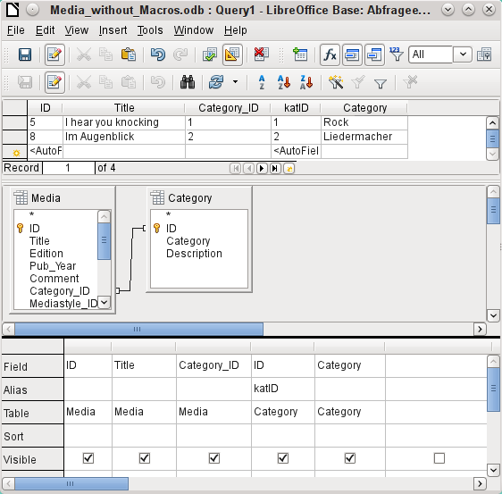
This query is editable as both primary keys are included and can be accessed in the tables without using an alias. A query that links several tables together also requires all primary keys to be present.
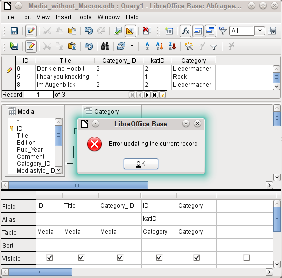
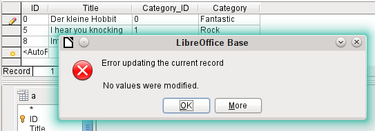
In a query that involves several tables, it is not possible to alter a foreign key field in one table that refers to a record in another table. In the record shown below, an attempt was made to change the category for the title “The Little Hobbit”. The Category_ID field was changed from 0 to 2. The change seemed to go through and the new category appeared in the record. However it proved impossible to save it.
However it is possible to edit the content of the corresponding category record, for example to replace “Fantasie” by “Fantasy”. The name of the category will then be altered for all records that are linked to this category.
SELECT "m"."ID", "m"."Title", "Category"."Category", "Category"."ID" AS "katID"
FROM "Media" AS "m", "Category"
WHERE "m"."Category_ID" = "Category"."ID";
In this query the Media table is accessed using an alias. The query cannot be edited.
In the above example, this problem is easily avoided. If, however, a correlated subquery (see page 1) is used, you need to use a table alias. A query is only editable in that case if it contains only one table in the main query.
In design view only one table appears. The Media table is given an alias so that the content of the Category_ID field can be accessed using a correlated subquery.
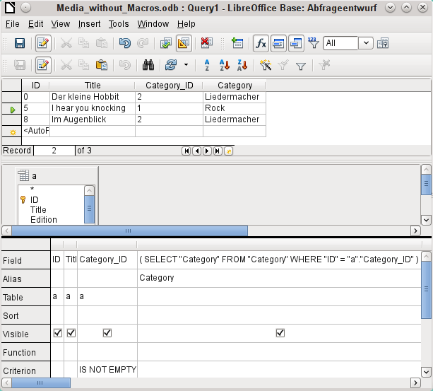
In a query like this, it is now possible to change the foreign key field Category_ID to another category. In the above example the Category_ID field is changed from 0 to 2. The title “The Little Hobbit“ is thus assigned to the category “Songwriter“.
However it is no longer possible to change a value in the field which has received its content via a correlated subquery. An attempted change in Category from ‘Fantasy’ to ‘Fantastic’ is shown. This change is not registered and cannot be saved either. In the table that the design view displays, the Category field is not present.
If you often use the same basic query but with different values each time, queries with parameters can be used. In principle queries with parameters function just like queries for a subform:
SELECT "ID", "Reader_ID", "Media_ID", "Loan_Date"
FROM "Loan"
WHERE "Return_Date" IS NULL AND "Reader_ID"=2;
This query shows only the media on loan to the reader with the number 2.
SELECT "ID", "Reader_ID", "Media_ID", "Loan_Date"
FROM "Loan"
WHERE "Return_Date" IS NULL AND "Reader_ID" =: Readernumber;
Now when you run the query, an entry field appears. It prompts you to enter a reader number. Whatever value you enter here, the media currently on loan to that reader will be displayed.
SELECT
"Loan"."ID",
"Reader"."LastName"||', '||"Reader"."FirstName",
"Loan"."Media_ID",
"Loan"."Loan_date"
FROM "Loan", "Reader"
WHERE "Loan"."Return_Date" IS NULL
AND "Reader"."ID" = "Loan"."Reader_ID"
AND "Reader"."LastName" LIKE '%' ||: Readername || '%'
ORDER BY "Reader"."LastName"||', '||"Reader"."FirstName" ASC;
This query is clearly more user-friendly than the previous one. It is no longer necessary to know the reader’s number. All you need to enter is part of the surname and all media on loan to matching readers are displayed.
If you replace
"Reader"."LastName" LIKE '%' || :Readername || '%'
by
LOWER("Reader"."LastName") LIKE '%' || LOWER(: Readername) || '%'
It no longer matters whether the name is entered in upper or lower case.
If the parameter in the above query is left empty, all versions of LibreOffice up to 4.4 would show all readers, since only in Version 4.4 does an empty parameter field read as NULL rather than as an empty string. If you don’t want this behavior, you must use a trick to prevent it:
LOWER ("Reader"."LastName") LIKE '%' || IFNULL(NULLIF (LOWER (:Readername), ''), '§§' ) || '%'
The empty parameter field returns an empty string and not a NULL to the query. Therefore the empty parameter field must be assigned the NULL property using NULLIF. Then, since the parameter entry does now yield NULL, it can be reset to a value that normally does not occur in any record. In the above example this is ‘$$’. This value of course will not be found in the search.
From Version 4.4, adaptations to this query technique are necessary:
LOWER ("Reader"."LastName") LIKE '%' || LOWER (:Readername) || '%'
must, in the absence of an entry, inevitably give for the combination:
'%' || LOWER (:Readername) || '%' a the NULL value.
To prevent this, add a further condition, that for an empty field, all values are actually shown:
(LOWER ("Reader"."LastName") LIKE '%' || LOWER (:Readername) || '%' OR: Readername IS NULL)
The whole thing needs to be put in brackets. Then either a name is searched for or, if the field is empty (NULL from LibreOffice 4.4), the second condition will apply.
When using forms, the parameter can be passed from the main form to a subform. However it sometimes happens that queries using parameters in subforms are not updated, if data is changed or newly entered.
Often it would be nice to alter the contents of list boxes using settings in the main form. So for example, we could prevent library media from being loaned to individuals who are currently banned from borrowing media. Unfortunately controlling list box settings in this personalized way by using parameters is not possible.
Subqueries built into fields can always only return one record. The field can also return only one value.
SELECT "ID", "Income", "Expenditure",
( SELECT SUM( "Income" ) - SUM( "Expenditure" )
FROM "Checkout") AS "Balance"
FROM "Checkout";
This query allows data entry (primary key included). The subquery yields precisely one value, namely the total balance. This allows the balance at the till to be read after each entry. This is still not comparable with the supermarket checkout form described in “Queries as a basis for additional information in forms” on page 1. Naturally it lacks the individual calculations of Total * Unit_price, but also the presence of the receipt number. Only the total sum is given. At least the receipt number can be included by using a query parameter:
SELECT "ID", "Income", "Expenditure",
( SELECT SUM( "Income" ) - SUM( "Expenditure" )
FROM "Checkout"
WHERE "Receipt_ID" = :Receipt_Number) AS "Balance"
FROM "Checkout" WHERE "Receipt_ID" =: Receipt_Number;
In a query with parameters, the parameter must be the same in both query statements if it is to be recognized as a parameter.
For subforms such parameters can be included. The subform then receives, instead of a field name, the corresponding parameter name. This link can only be entered in the properties of the subform, and not when using the Wizard.
Note
Subforms based on queries are not automatically updated on the basis of their parameters. It is more appropriate to pass on the parameter directly from the main form.
Using a still more refined query, an editable query allows you to even carry the running balance for the till:
SELECT "ID", "Income", "Expenditure",
( SELECT SUM( "Income" ) - SUM( "Expenditure" )
FROM "Checkout"
WHERE "ID" <= "a"."ID" ) AS "Balance"
FROM "Checkout" AS "a"
ORDER BY "ID" ASC
The Checkout table is the same as Table "a". "a" however yields only the relationship to the current values in this record. In this way the current value of ID from the outer query can be evaluated within the subquery. Thus, depending on the ID, the previous balance at the corresponding time is determined, if you start from the fact that the ID, which is an autovalue, increments by itself.
Note
If the subquery is to be filtered for content using the query editor’s filter function, this currently only works if you use double brackets instead of single ones at the beginning and end of the subquery: ((SELECT ….)) AS "Saldo"
A query is required to set a lock against all readers who have received a third overdue notice for a medium.
SELECT "Loan"."Reader_ID", '3rd Overdue – the reader is blacklisted' AS "Lock"
FROM
(SELECT COUNT( "Date" ) AS "Total_Count", "Loan_ID"
FROM "Recalls" GROUP BY "Loan_ID") AS "a",
"Loan"
WHERE "a"."Loan_ID" = "Loan"."ID" AND "a"."Total_Count" > 2
First let us examine the inner query, to which the outer query relates. In this query the number of date entries grouped by the foreign key Loan_ID is determined. This must not be made dependent on the Reader_ID, as that would cause not only three overdue notices for a single medium but also three media with one overdue notice each to be counted. The inner query is given an alias so that it can be linked to the Reader_ID from the outer query.
The outer query relates in this case only to the conditional formula from the inner query. It shows only a Reader_ID and the text for the Lock field when the "Loan"."ID" and "a"."Loan_ID" are equal and "a"."Total_Count" > 2.
In principle all fields in the inner query are available to the outer one. So for example the sum "a"."Total_Count" can be merged into the outer query to give the actual fines total.
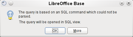
However it can happen, in the Query Design dialog, that the Design View Mode no longer works after such a construction. If you try to open the query for editing again you get the following warning:
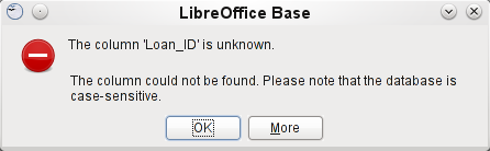
If you then open the query for editing in SQL view and try to switch from there into the Design View, you get the error message:
The Design View Mode cannot find the field contained in the inner query "Loan_ID", which governs the relationship between the inner and outer queries.
When the query is run in SQL Mode, the corresponding content from the subquery is reproduced without error. Therefore you do not have to use direct SQL mode in this case.
The outer query used the results of the inner query to produce the final results. These are a list of the "Loan_ID" values that should be locked and why. If you want to further limit the final results, use the sort and filter functions of the graphical user interface.
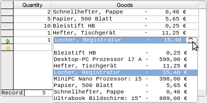
The following screenshots show how the different way to a query result with subqueries can go. Here a query to a stock database is trying to determine what the customer needs to pay at the till. The individual prices are multiplied by the number of items bought giving a subtotal. Then the sum of these subtotals needs to be determined. All this needs to be editable so that the query can be used as the basis for a form.
Figure 5: Query using two tables. To make it editable, both primary keys must be included.
Note
Because of Bug 61871, Base does not update the partial result automatically.
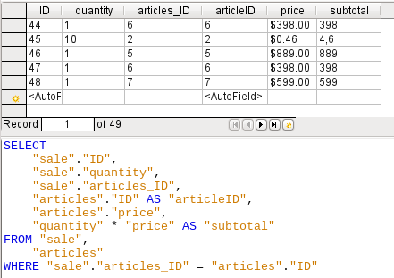
Figure 6: The Articles table is moved into a subquery, which is created in the table area (after the “FROM” term) and given an alias. Now the primary key of the Articles table is no longer strictly necessary to make the query editable.
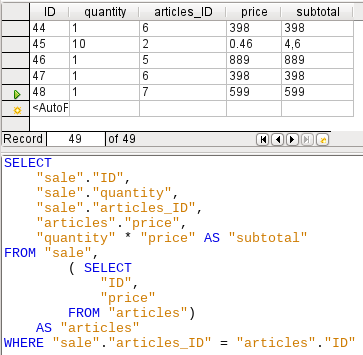
Figure 7: Now the calculated sum must appear in the query. Already the simple query for the calculation sum is not editable so it is grouped and summed here.
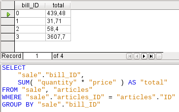
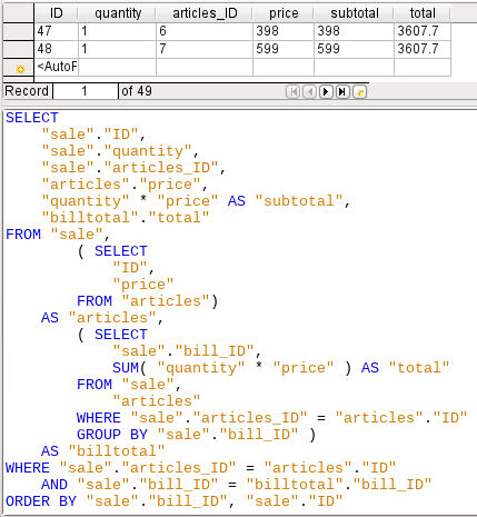
Figure 8: With the second subquery the seemingly impossible becomes possible. The previous query is inserted as a subquery into the table definition of the main query (after “FROM”). As a result, the whole query remains editable. In this case entries are only possible in the “Sum” and “WarID” columns. This is subsequently made clear in the query form.
When data is searched for over a whole database, the use of simple form functions often leads to problems. A form refers after all to only one table, and the search function moves only through the underlying records for this form.
Getting at all the data is simpler when you use queries, which can provide a picture of all the records. The section on “Relationship definition in the query” suggests such a query construction. This is constructed for the example database as follows:
SELECT "Media"."Title", "Subtitle"."Subtitle", "Author"."Author"
FROM "Media"
LEFT JOIN "Subtitle"
ON "Media"."ID" = "Subtitle"."Media_ID"
LEFT JOIN "rel_Media_Author"
ON "Media"."ID" = "rel_Media_Author"."Media_ID"
LEFT JOIN "Author"
ON "rel_Media_Author"."Author_ID" = "Author"."ID"
Here all Titles, Subtitles, and Authors are shown together.
The Media table contains a total of 9 Titles. For two of these titles, there are a total of 8 Subtitles. Without a LEFT JOIN, both tables displayed together yield only 8 records. For each Subtitle, the corresponding Title is searched for, and that is the end of the query. Titles without Subtitle are not shown.
Now to show all Media including those without a Subtitle: Media is on the left side of the assignment, Subtitle on the right side. A LEFT JOIN will show every Title from Media, but only a Subtitle for those that have a Title. Media becomes the decisive table for determining which records are to be displayed. This was already planned when the table was constructed (see Chapter 3, Tables). As Subtitles exist for two of the nine Titles, the query now displays 9 + 8 – 2 = 15 records.
Note
The normal linking of tables, after all tables have been listed, follows the keyword WHERE.
If there is a LEFT JOIN or a RIGHT JOIN, the assignment is defined directly after the two table names using ON. The sequence is therefore always
Table1 LEFT JOIN Table2 ON Table1.Field1 = Table2.Field1 LEFT JOIN Table3 ON Table2.Field1 = Table3.Field1...
Two Titles of the Media table do not yet have an Author entry or a Subtitle. At the same time one Title has a total of three Authors. If the Author table is linked without a LEFT JOIN, the two Media without an Author will not be shown. But as one medium has three authors instead of one, the total number of records displayed will still be 15.
Only by using LEFT JOIN will the query be instructed to use the Media table to determine which records to show. Now the records without Subtitle or Author appear again, giving a total of 17 records.
Using appropriate Joins usually increases the amount of data displayed. But this enlarged data set can easily be scanned, since authors and subtitles are displayed in addition to the titles. In the example database, all of the media-dependent tables can be accessed.
Views in SQL are quicker than queries, especially for external databases, as they are anchored directly into the database and the server returns only the results. By contrast queries are first sent to the server and processed there.
If a new query relates to another query, the SQL view in Base makes the other query look like a table. If you create a View from it, you can see that you are actually working with a subquery (Select used within another Select). Because of this, a Query 2 that relates to another Query 1 cannot be run by using Edit > Run SQL command directly, since only the graphical user interface and not the database itself knows about Query 1.
The database gives you no direct access to queries. This also applies to access using macros. Views, on the other hand, can be accessed from both macros and tables. However, no records can be edited in a view. (They must be edited in a table or form.)
Tip
A query created using Create Query in SQL View has the disadvantage that it cannot be sorted or filtered using the GUI. There are therefore limits to its use.
A View on the other hand can be managed in Base just like a normal table – with the exception that no change in the data is possible. Here therefore even in direct SQL-commands all possibilities for sorting and filtering are available.
In addition, the formatting of columns in a view is retained when the database is closed, unlike columns in a query.
Views are a solution for many queries, if you want to get any results at all. If for example a Subselect is to be used on the results of a query, create a View that gives you these results. Then use the subselect on the View. Corresponding examples are to be found in Chapter 8, Database Tasks.
Creating a View from a query is rather easy and straightforward.
1) Click the Table object in the Database section.
2) Click Create View.
3) Close the Add Table dialog.
4) Click the Design View On/Off icon. (This is the SQL Mode for a View.)
5) Getting the SQL for the View:
a) Edit the query in SQL View.
b) Use Control+A to highlight the query’s SQL.
c) Use Control+C to copy the SQL.
6) In the SQL Mode of the View, use Control+V to paste the SQL.
7) Close, save, and name the View.
Queries are also used to calculate values. Sometimes the internal HSQLDB database produces apparent errors, which on closer examination turn out to be logically correct interpretations of the data. There are also rounding problems, which can easily cause confusion.
Times within HSQLDB are formatted correctly only up to a difference of 23:59:59 hours. If several times are to be added, for example to calculate hours worked, another way must be found. Here there are several complicated approaches:
Time is directly expressed only as a total of minutes or even seconds. Advantage: the values allow subsequent problem-free calculation.
The time is split into hour, minute and second parts and reassembled as text using ‘:’ as a separator. Advantage: the text appears in queries as properly formatted time from the beginning.
The time is created as a decimal number. A day is 1, an hour is 1/24 and so on. Advantage: the values can subsequently be reformatted as time in the query and presented as a formattable form field.
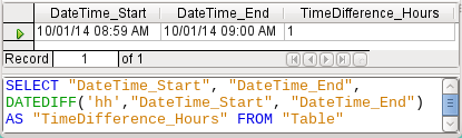
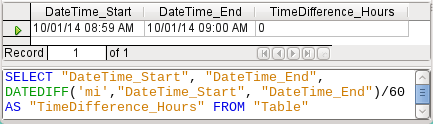
DATEDIFF allows time intervals to be determined. It explicitly asks for the difference that is to be determined. In the above example, minutes have not been requested, but all elements that are greater than a minute are considered. That gives one hour (!) as the difference between 8:59 and 9:00. By contrast, a date difference is calculated as a time difference in hours. If for example the Date_time_end field is set to 2.10.14 09:00, that is calculated as 25 hours.
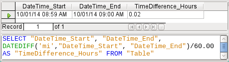
If instead the time interval is calculated in minutes and then divided by 60, the time difference in hours becomes zero. This looks more like the correct value, except: where did that one minute go?
The time interval has been given as an integer. An integer has been divided by an integer. The result of the query in such cases must also be an integer, not a decimal number. This can easily be corrected. The time difference in minutes is divided by a decimal number with two decimal places (60.00). This gives a result that also has two decimal places. 0.02 hours is still not exactly one minute but is much closer to it than before. The number of decimal places could be increased by using more zeros. A period of 0.016 is a closer approximation still, but later calculation errors cannot always be excluded.
Instead of having to work with lots of added zeros, the data type of DATEDIFF can be influenced directly. Using (CONVERT(DATEDIFF('mi', "Date_time_start", "Date_time_end"),DECIMAL(50,49)))/60 you can achieve an accuracy of 49 decimal places.
When using calculation functions you must always understand that the data types in HSQLDB have only a limited precision. However many decimal places you use, the fact remains that intermediate results involving a time count can only be used to a limited extent for further calculations.
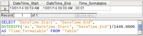
If a time value is subsequently to be used in a form or report as a formatted time, you must ensure that the day is valid as a basis for the time format.
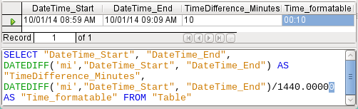
Here the difference is calculated in minutes. The result is given as a fraction of a day. One day has 60 * 24 minutes. If you simply divided by 1440, the result would be zero, so once again you need to give the decimal places explicitly. It then appears as a formatted time of 0 hours and 1 minute.
The format code for a time longer than one day is [HH]:MM. If you use the wrong format, a time difference of 1 day and 1 minute could be shown as only 1 minute.
The error fiend strikes again! A time difference of 10 minutes should not show up as 9 minutes when correctly formatted. To find out where the problem lies, we need to consider exactly how the calculation is done:
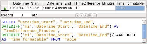
1) 10/1440 = 0.00694. The result is rounded down to 0.0069 because only four decimal places were specified.
2) 0.0069 * 1440 = 9.936 minutes, which is 9 minutes 56.16 seconds. And seconds are not displayed in the chosen format!
Lengthening the divisor by just one decimal place (from 1440.0000 to 1440.00000) cures this error. Now the rounding is to 0.00694. 0.00694*1440 gives 9.9936 which is 59.616 seconds. The number of seconds is rounded up to 60 seconds, so the 9 minutes have 1 minute added, making 10 minutes in all.
Here too there might be further problems. Might there be further decimal places which, when formatted, do not yield 1 minute? To settle this, a short calculation using Calc with similarly rounded figures can help. Column A contains a sequence of numbers from 1 (for the minutes). Column B contains the formula =ROUND(A1/1440;4) and is formatted to show hours and minutes. If this continues downwards, we can see, next to 10 minutes in column A, 00:09 in column B. Similarly for 28 minutes, etc. If you round to 5 places, these errors disappear.
However nice it might be to have a suitably formatted display in a form, you need to be aware that you are dealing with rounded values which are not suitable for further use in blindly mechanical calculations. If a value needs to be used for further calculation, it is better to use only a representation of time difference in the smallest available units, in this case minutes.