Calc Guide 24.8
Chapter 11 Data Analysis
Using Scenarios, Goal Seek, Solver, Statistics, others
This document is Copyright © 2025 by the LibreOffice Documentation Team. Contributors are listed below. You may distribute it and/or modify it under the terms of either the GNU General Public License (https://www.gnu.org/licenses/gpl.html), version 3 or later, or the Creative Commons Attribution License (https://creativecommons.org/licenses/by/4.0/), version 4.0 or later.
All trademarks within this guide belong to their legitimate owners.
|
Edward Olson |
Lisa Samy |
Olivier Hallot |
|
Barbara Duprey |
Jean Hollis Weber |
John A Smith |
|
Kees Kriek |
Zachary Parliman |
Olivier Hallot |
|
Steve Fanning |
Leo Moons |
Felipe Viggiano |
|
Skip Masonsmith |
B. Antonio Fernández |
|
Please direct any comments or suggestions about this document to the Documentation Team’s forum at https://community.documentfoundation.org/c/documentation/loguides/ (registration is required) or send an email to: loguides@community.documentfoundation.org.
Note
Everything you send to a forum, including your email address and any other personal information that is written in the message, is publicly archived and cannot be deleted. Emails sent to the forum are moderated.
Published January 2025. Based on LibreOffice 24.8 Community.Other versions of LibreOffice may differ in appearance and functionality.
Some keystrokes and menu items are different on macOS from those used in Windows and Linux. The table below gives some common substitutions for the instructions in this document. For a detailed list, see the application Help and Appendix A (Keyboard Shortcuts) to this guide.
|
Windows or Linux |
macOS equivalent |
Effect |
|
Tools > Options on Menu bar |
LibreOffice > Preferences on Menu bar |
Access to setup options |
|
Right-click |
Ctrl+click and/or right-click depending on computer setup |
Opens a context menu |
|
Ctrl or Control |
⌘ and/or Cmd or Command, depending on keyboard |
Used with other keys |
|
Alt |
⌥ and/or Alt or Option depending on keyboard |
Used with other keys |
Once you are familiar with functions and formulas described in the previous chapter, the next step is to learn how to use Calc’s automated processes to quickly perform useful analysis of your data.
Besides formulas and functions, Calc offers various tools for data processing. These tools include features for copying and reusing data, creating subtotals, conducting what-if analysis, and performing statistical analysis. You can find them under the Tools and Data menus on the Menu bar. While not essential for using Calc, these tools can save you time and effort when managing large data sets or preserving your work for future review.
Note
A related tool, the Pivot Table, is not discussed here due to its complexity, which warrants a dedicated chapter. For more information, refer to Chapter 10, Using Pivot Tables.
The Consolidate tool allows you to combine and aggregate data spread across one or more sheets. This tool is useful if you need to quickly summarize a large, scattered set of data for review. For example, you could use it to consolidate multiple department budgets from different sheets into a single company-wide budget contained in a master sheet.
To consolidate data:
Open the document containing the cell ranges to be consolidated.
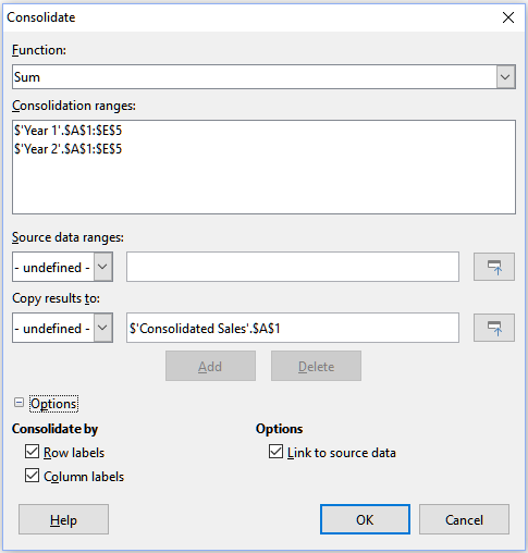
Select Data > Consolidate on the Menu bar to open the Consolidate dialog (Figure 1).
Click on the Source data ranges field, then type a reference to a source data range, a named range, or select it with the mouse. Use the associated Shrink / Expand button if you need to minimize the dialog while you select the range. Alternatively, select a named range from the drop-down list to the left of the field.
Click Add. The selected range is added to the Consolidation ranges list.
To delete an entry in the Consolidation ranges list, select it and click Delete. The deletion is carried out without further confirmation.
Click on the Copy results to field, then type a reference to the first cell of the target range or select it with your mouse. You can also select a named range in the drop-down list to the left of the field.
Select a function to aggregate your data in the Function drop-down list. The default is Sum. Other available functions are Count, Average, Max, Min, Product, Count (numbers only), StdDev (sample), StDevP (population), Var (sample), and VarP (population).
Click OK to consolidate the ranges. Calc runs the function from step 8) on your source data ranges and populates the target range with the results.
Tip
If you are consolidating the same cell ranges repeatedly, consider converting them into reusable named ranges to make the process easier. For more information about named ranges, see Chapter 14, Calc as a Database.
Figure 1: Consolidate dialog
In the Consolidate dialog, expand the Options section to access the settings shown in Figure 2.
Figure 2: Consolidate dialog – Options section
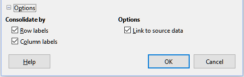
Consolidate by
Row labels – Consolidates rows by matching label. If this option is unchecked, the tool will consolidate rows by position instead.
Column labels – Works the same as Row labels, but with columns instead.
Options
Note
If you use the Link to source data option, each source link is inserted into the target range, then ordered and hidden from view. Only the final results of consolidation are displayed by default.
Figure 3, Figure 4, and Figure 5 show a simple example of consolidation using a spreadsheet with the sheets Year 1, Year 2, and Consolidated Sales. Figure 3 shows the contents of the Year 1 sheet, with sales figures by region for each of the four product colors.
Figure 3: Year 1 sales by region
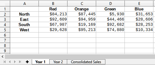
Figure 4 shows the Year 2 sheet, sales figures by region for each of four product colors. Note the different ordering of row and column labels between the two figures.
Figure 4: Year 2 sales by region
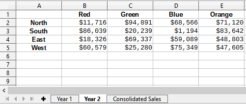
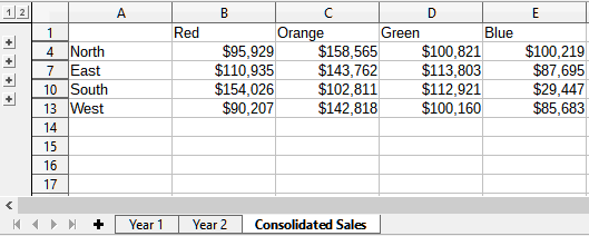
Figure 5 shows the consolidated sales data, created by using the Consolidate dialog settings shown in Figure 2. Note that because the Link to source data option was selected, clicking on the plus sign (+) indicators to the left of the data will reveal formula links back to the source ranges.
The source ranges and target range are saved as part of the document. If you later open a document with consolidated ranges, they will still be available in the Consolidation ranges list of the Consolidate dialog.
Figure 5: Consolidated sales by region
Calc offers two methods of creating subtotals: the SUBTOTAL function and the Subtotals tool.
The SUBTOTAL function is listed under the Mathematical category of the Function Wizard, and the Functions deck of the Sidebar, which are described in Chapter 8, Using Formulas and Functions. SUBTOTAL is a relatively limited method for generating a subtotal, and works best if used with only a few categories.
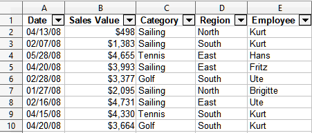
To illustrate how to use the SUBTOTAL function, we use the sales data sheet shown in Figure 6. The AutoFilter function is already applied to the sales data, as indicated by the down arrow buttons at the head of each column. AutoFilters are described in Chapter 2, Entering and Editing Data.
Figure 6: Sales data with AutoFilter applied (only the first few rows are shown)
To create a summation subtotal for the Sales Value field using the Function Wizard:
Select the cell to contain a subtotal. Typically, this cell is at the bottom of the column being subtotaled, which, for our example, is the Sales Value column.
Use one of the following methods to open the Function Wizard dialog (Figure 7):
Select Insert > Function on the Menu bar
Click the Function Wizard icon on the Formula bar
Press Ctrl+F2
Figure 7: Function Wizard dialog
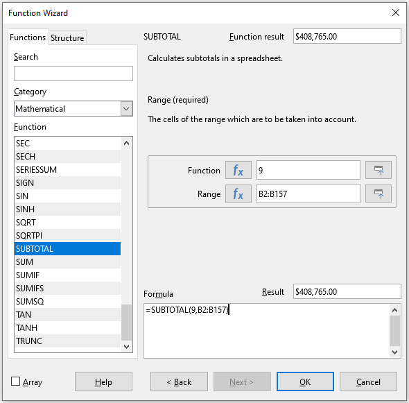
Select SUBTOTAL in the Function list of the Function Wizard dialog and click Next.
Enter the numeric code of a function into the Function field on the right side of the dialog. This code must be a value in the range 1 to 11, or 101 to 111, with the meaning of each value shown in Table 1.
Note
Values 1 to 11 include hidden values in the calculated subtotal, while values 101 to 111 do not. Hiding and showing data is described in Chapter 2, Entering and Editing Data. Filtered-out cells are always excluded by the SUBTOTAL function.
Table 1: SUBTOTAL function numbers
|
Function index (includes hidden values) |
Function index (ignores hidden values) |
Function |
|
1 |
101 |
AVERAGE |
|
2 |
102 |
COUNT |
|
3 |
103 |
COUNTA |
|
4 |
104 |
MAX |
|
5 |
105 |
MIN |
|
6 |
106 |
PRODUCT |
|
7 |
107 |
STDEV |
|
8 |
108 |
STDEVP |
|
9 |
109 |
SUM |
|
10 |
110 |
VAR |
|
11 |
111 |
VARP |
Click on the Range field, then type a reference to the Sales Value range or select the cells with your mouse (Figure 7). Use the Shrink / Expand button if you need to temporarily minimize the dialog while selecting the cells.
Click OK to close the Function Wizard dialog. The cell you selected in step 1) now contains the total sales value.
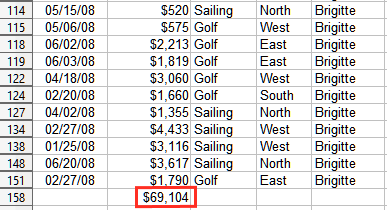
Click on the AutoFilter down arrow button at the top of the Employee column and remove all marks from the filter area except those next to Brigitte and (empty). The cell that you selected in step 1) should now reflect the sum of all of Brigitte’s sales (Figure 8).
Note
If the cell range used to calculate a subtotal contains other subtotals, these subtotals will not be counted in the final one. Similarly, if you use this function with AutoFilters, only the data satisfying the current filter selections will be displayed. Any filtered-out data is ignored.
Figure 8: SUBTOTAL result for Brigitte’s sales
Calc offers the Subtotals tool as a more comprehensive alternative to the SUBTOTAL function. In contrast to SUBTOTAL, which only works on a single array, the Subtotals tool can create subtotals for up to three arrays arranged in labeled columns. It also groups subtotals by category and sorts them automatically, thereby eliminating the need to apply AutoFilters and filter categories by hand.
To insert subtotal values into a sheet:
Select the cell range for the subtotals that you want to calculate, and remember to include the column heading labels. Alternatively, click on a single cell within your data to allow Calc to automatically identify the range.
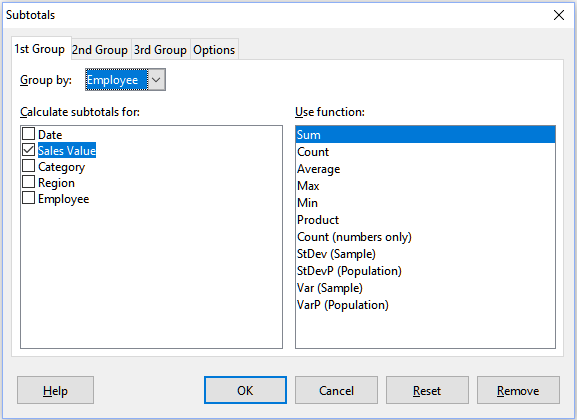
Select Data > Subtotals on the Menu bar to open the Subtotals dialog (Figure 9).
In the Group by drop-down list on the 1st Group tab, select a column by its label. Entries in the cell range from step 1) will be grouped and sorted by matching values in this column.
In the Calculate subtotals for box on the 1st Group tab, select a column containing values to be subtotaled. If you later change values in this column, Calc will automatically recalculate the subtotals.
In the Use function box on the 1st Group tab, select a function to calculate the subtotals for the column selected in step 4).
Repeat steps 4) and 5) to create subtotals for other columns on the 1st Group tab.
You can create two more subtotal categories by using the 2nd Group and 3rd Group tabs and repeating steps 3) to 6). If you do not want to add more groups, then leave the Group by list for each page set to “- none -”.
Click OK. Calc will add subtotal and grand total rows to your cell range.
Figure 9: Subtotals dialog
For our sales data example, a partial view of the results is shown in Figure 10. The group settings are identified in Table 2.
Table 2: Group settings used on Subtotals dialog for example sales data
|
Tab |
Group by |
Calculate subtotals for |
Use function |
|
1st Group |
Employee |
Sales Value |
Sum |
|
2nd Group |
Category |
Sales Value |
Sum |
|
3rd Group |
- none - |
- |
- |
When you use the Subtotals tool, Calc inserts an outline to the left of the row number column. This outline represents the hierarchical structure of your subtotals, and can hide or show data at different levels in the hierarchy using the numbered column indicators at the top of the outline or the group indicators, denoted by plus (+) and minus (-) signs.
This feature is useful if you have many subtotals, as you can simply hide low-level details, such as individual entries, to produce a high-level summary of your data. For more information on how to use outlines, see Chapter 2, Entering and Editing Data.
To turn off outlines, select Data > Group and Outline > Remove Outline on the Menu bar. To reinstate them, select Data > Group and Outline > AutoOutline.
Figure 10 shows the outline for our sales data example.
Figure 10: Partial outlined view of sales data example with subtotals
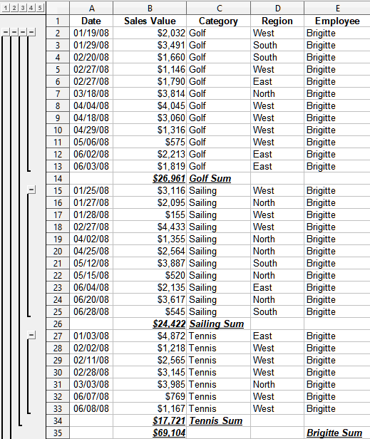
Column 1 represents the highest group level, the grand total over all employees. Outline columns 2 to 5 show descending group levels as follows:
Column 2 represents the grand total over all categories.
Column 3 represents the total for each employee.
Column 4 represents the total for each category for an individual employee.
Column 5 shows individual entries.
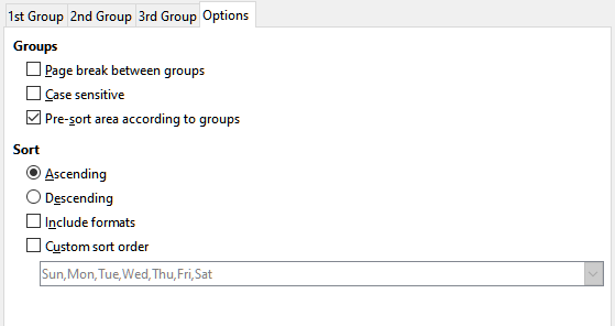
Click on the Options tab of the Subtotals dialog to access the following settings:
Groups
Page break between groups – inserts page breaks between each subtotal group so that each group displays on a separate page when you print the data.
Case sensitive – prevents the tool from grouping entries by data labels that differ by case. In our sales data example, entries with “Brigitte” and “brigitte” under the Employee column will not match if this option is selected.
Pre-sort area according to groups – sorts entries by group before calculating subtotals. Disabling this option prevents the tool from grouping matching entries together. As a result, distinct subtotals will be created for matching entries if they do not appear on consecutive rows. For example, two entries under the “Golf” category will not count towards the same group subtotal if there is an entry for “Tennis” in between them.
Figure 11: Options tab of the Subtotals dialog
Sort
Ascending or Descending – sorts entries by value from lowest to highest and highest to lowest, respectively. You can modify these sort rules by using Data > Sort on the Menu bar. For more detail, see Chapter 2, Entering and Editing Data.
Include formats – carries over formatting, such as the currency format, from the data to the corresponding subtotals.
Custom sort order – sorts your data according to one of the predefined custom sorts defined in Tools > Options > LibreOffice Calc > Sort Lists on the Menu bar. For more details about custom sort lists, see Chapter 2, Entering and Editing Data.
In the Subtotals dialog, use the Reset button to undo any changes made on the current tab. Use the Remove button to remove any subtotals that have already been created using the Subtotals tool. Use these features with care, as no confirmation dialog is displayed.
Scenarios are cell ranges that have been saved and named. They can be used to answer “what-if” questions about your data. You can create multiple scenarios for the same calculation set, then quickly swap between them to view the outcomes of each. This feature is useful if you need to test the effects of different conditions on your calculations, but do not want to deal with repetitive manual data entry. For example, if you wanted to test different interest rates for an investment, you could create scenarios for each rate, then switch between them to find out which rates work the best for you.
To create a new scenario:
Select the cells that contain the values that will change between scenarios. To select multiple ranges, hold down the Ctrl key as you click. You must select at least two cells.
Choose Tools > Scenarios on the Menu bar to open the Create Scenario dialog (Figure 12).
Figure 12: Create Scenario dialog
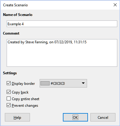
Enter a name for the new scenario in the Name of Scenario field.
Tip
When naming a new scenario, use a unique name that clearly identifies and distinguishes it from other scenarios. The default name suggested by Calc may not be the best choice, especially if you have a large set of scenarios.
Optionally, add information to the Comment field. The example in Figure 12 shows the default comment.
Click OK to close the dialog. The new scenario is automatically activated upon creation.
Repeat steps 1) to 5) to create additional scenarios. Select the same cell range that you used for the first scenario to have multiple scenarios for the same calculations.
Tip
To keep track of which calculations are dependent on your scenarios, use Tools > Detective > Trace Dependents on the Menu bar after highlighting your scenario cells. For more information about the Detective tool, see Chapter 8, Using Formulas and Functions.
The Settings section of the Create Scenario dialog (Figure 13) contains the following options:
Figure 13: Create Scenario dialog – Settings
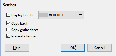
Display border
Figure 14: Scenario cell range with border
Copy back
Caution
When creating a new scenario from the cells of a scenario with Copy back enabled, be careful not to overwrite the old scenario. To avoid this situation, create the new scenario with Copy back enabled first, then change its values only once it is active.
Copy entire sheet
Prevent changes
Scenarios have two aspects that can be altered independently:
Scenario properties (that is, its settings)
Scenario cell values
The extent to which these aspects can be changed depends on the active scenario's properties and the current sheet and cell protections. For more detail about sheet and cell protections, see Chapter 2, Entering and Editing Data.
Table 3 summarizes how sheet protection and the Prevent changes option affect your ability to change scenario properties.
Table 3: Changing scenario properties
|
Sheet protection |
Prevent changes |
Property changes |
|
On |
On |
No scenario properties can be changed. |
|
On |
Off |
Display border and Copy back can be changed. Prevent changes and Copy entire sheet cannot be changed. |
|
Off |
Any setting |
All scenario parameters except for Copy entire sheet can be changed. In this case, the Prevent changes option has no effect. |
Table 4 summarizes the interaction of various settings in making changes to scenario cell values.
Table 4: Changing scenario cell values
|
Sheet protection |
Scenario cell protection |
Prevent changes |
Copy back |
Change allowed |
|
On |
Off |
On |
On |
Scenario cell values cannot be changed. |
|
On |
Off |
Off |
On |
Scenario cell values can be changed, and the scenario is updated. |
|
On |
Off |
Any setting |
Off |
Scenario cell values can be changed, but the scenario is not updated due to the Copy back setting. |
|
On |
On |
Any setting |
Any setting |
Scenario cell values cannot be changed. |
|
Off |
Any setting |
Any setting |
Any setting |
Scenario cell values can be changed and the scenario is updated or not, depending on the Copy back setting. |
Scenarios that have been added to a spreadsheet may be viewed using the Navigator. To open a scenario, select View > Navigator from the Menu bar, then click on the Scenarios icon in the Navigator and choose a scenario from the list (Figure 15). All defined scenarios are listed along with the comments entered when each scenario was created. You can also use the equivalent features in the Navigator deck of the Sidebar. For more information about the Navigator, refer to Chapter 1, Introduction.
Figure 15: Scenarios in the Navigator
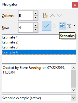
To apply a scenario to the current sheet, double-click the scenario name in the Navigator.
To delete a scenario, right-click the name in the Navigator and choose Delete, or press the Delete key after selecting it. A confirmation dialog will be displayed.
To edit a scenario, right-click the name in the Navigator and choose Properties. Calc displays the Edit Scenario dialog, which is similar to the Create Scenario dialog (Figure 12).
Similar to scenarios, the Multiple Operations tool conducts what-if analysis on your calculations. However, unlike scenarios that represent individual sets of values for multiple formula variables, this tool uses a range of values for just one or two variables. It then applies one or more formulas to generate a corresponding range of solutions. Because each solution is linked to one or two variable values, both the variable and solution ranges can be easily organized in a tabular format. Consequently, the Multiple Operations tool is ideal for producing data that is easy to read, share, or visualize using graphs.
Tip
Exercising good organization can make using this tool relatively painless. For example, we recommend keeping your data together on one sheet and using labels to identify your formulas, variables, and table ranges.
The simplest way to learn how to use the Multiple Operations tool is by starting with one formula and one variable. For guidance on using the tool with multiple formulas or with two variables, refer to the sections "Calculating with several formulas simultaneously" and "Multiple operations with two variables" below, respectively.
To use the Multiple Operations tool with one formula and one variable:
In the cells of a worksheet, enter a formula and at least one variable that it uses.
In the same worksheet, enter values into a cell range that occupies a single column or row. These values are used for one of the variables of the formula that you defined in step 1).
With the mouse, select the range containing both the variable range that you defined in step 2) and the adjacent empty cells that follow it. Depending on how your variable range is arrayed, these empty cells will either be in the column to the right (if the range is in a column) or in the row immediately below (if it is in a row).
Select Data > Multiple Operations on the Menu bar to open the Multiple Operations dialog (Figure 16).
Figure 16: Multiple Operations dialog
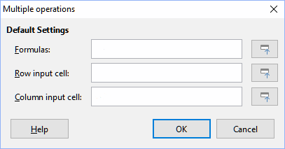
Click on the Formulas field and type a cell reference to the formula you defined in step 1) or select the cell with the mouse. Use the associated Shrink / Expand button if you need to minimize the dialog while selecting the cell.
If the range from step 2) is arrayed in a column, then click on the Column input cell field and type a cell reference to the variable that you want to use or select the cell with the mouse. If the range is in a row, then use the Row input cell field instead.
Click OK to run the tool. The Multiple Operations tool will generate its results in the empty cells that you selected in step 3). Each result value corresponds to the variable value adjacent to it, and together they form the entries of a results table.
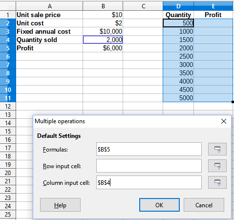
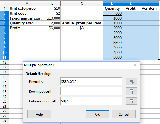
Using the Multiple Operations tool is best explained by example. Suppose that you produce toys that you sell for $10 each (cell B1 of a worksheet). Each toy costs $2 to make (B2), and you have a fixed annual cost of $10,000 (B3). What is the minimum number of toys that you must sell to break even? Suppose that our initial estimate of quantity sold is 2,000 (B4).
Figure 17: Inputs to Multiple Operations tool for one formula, one variable
To answer this question:
Enter the following formula into B5: =B4*(B1-B2)-B3. This formula represents the equation Profit = Quantity * (Selling price – Direct costs) – Fixed costs. With this equation, our initial quantity produces a $6,000 profit, which is higher than the break-even point.
In D2:D11, enter a range of alternate quantities from 500 to 5000 in steps of 500.
Select the range D2:E11 to define the results table. This range includes the alternate quantity values (column D) and the empty results cells (column E).
Select Data > Multiple Operations on the Menu bar to open the Multiple Operations dialog.
Using the Formulas field, select the cell B5.
Figure 18: Results of Multiple Operations tool for one formula and one variable
Using the Column input cell field, select the cell B4 to set the quantity as the variable for our calculations. Figure 17 shows the worksheet and Multiple Operations dialog at this point.
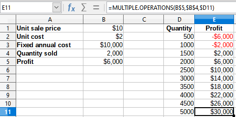
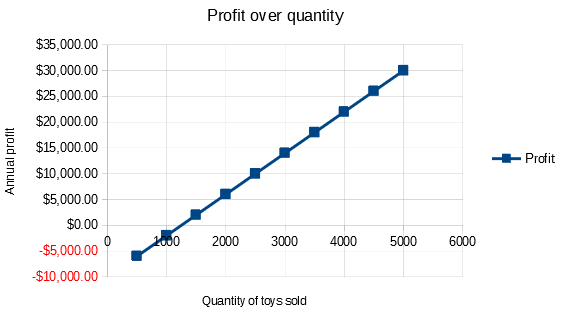
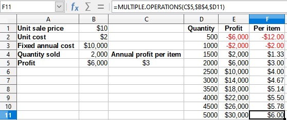
Click OK. The profits for the different quantities are now shown in column E (Figure 18). We can see that the break-even point is between 1000 and 1500 toys sold – namely, 1250. Figure 18 shows an XY (Scatter) chart showing the profit as a function of quantity.
Figure 19: XY (Scatter) plot of profit over quantity of toys sold (visualization example)
Using the Multiple Operations tool with multiple formulas follows nearly the same process as with one formula, but with two important differences:
For each formula that you add, you must also add a corresponding column or row to the results table to contain the output of that formula.
How you initially arrange your formulas determines how their results will be displayed in the results table. For example, if you arrange the formulas A, B, and C in a single row in that order, then Calc will generate the results of A in the first results table column, the results of B in the second column, and the results of C in the third.
Note
The Multiple Operations tool only accepts formulas arranged in a single row or column, depending on how your results table is oriented. If the table is column-oriented – that is, the way it is in our sales data example – then your formulas must be arranged in a row. If the table is row-oriented, then your formulas must be in a column.
Caution
Be careful not to add empty cells between formulas, as they will create gaps in the results table and may cause some results not to appear if you don't select enough rows or columns for the table.
Using our sales data example, suppose that we want to calculate the annual profit per item sold in addition to the annual overall profit. To calculate the results:
In the sheet from the previous example, delete the results in column E.
Enter the following formula in C5: =B5/B4. You are now calculating the annual profit per item sold.
Select the range D2:F11 for the results table. Column F will contain the results of the annual profit per item formula in C5.
Select Data > Multiple Operations on the Menu bar to open the Multiple Operations dialog.
Using the Formulas field, select the range B5:C5.
Using the Column input cell field, select the cell B4. Figure 20 shows the worksheet and the dialog at this point.
Figure 20: Inputs to Multiple Operations tool for one variable and two formulas
Click OK. Now the profits are listed in column E and the annual profit per item in column F.
Figure 21: Results of Multiple Operations tool for one variable and two formulas
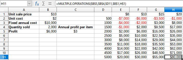
When using the Multiple Operations tool with two variables, it generates a two-dimensional results table. Each variable defines one dimension of the table: the alternate values for one variable form the row headings, while the values for the other variable form the column headings. Each cell in the table represents a unique combination of row and column values, with the results calculated based on these paired values.
Since two variables are involved, you must specify both the Column input cell and Row input cell fields. The order of these inputs is critical: the Column input cell field determines the row heading values, and the Row input cell field determines the column heading values.
Tip
Since column headings are in a row at the top of the table, they correspond to the Row input cell field. Likewise, row headings are in a column, so they correspond to the Column input cell field.
Note
If you use two variables, the Multiple Operations tool will not work with multiple formulas. It will allow you to enter the extra formulas, but will not generate the expected results for any formula beyond the first.
Using our sales example, suppose that in addition to varying the quantity of toys sold, you also want to vary the unit sale price as well. To calculate the results:
Expand the sales data table by entering $8, $10, $15 and $20 in the range E1:H1.
Select the range D1:H11 for the results table.
Select Data > Multiple Operations on the Menu bar to open the Multiple Operations dialog.
Using the Formulas field, select cell B5.
Using the Row input cell field, select cell B1. The column headings – $8, $10, $15 and $20 – are now linked to the unit sale price variable defined in cell B1.
Using the Column input cell field, select cell B4. The row headings – 500, 1000, ... , 5000 – are now linked to the quantity sold variable defined in cell B4. Figure 22 shows the worksheet and dialog at this point.
Click OK. The profits for the different sale prices and quantities are now shown in the range E2:H11 (Figure 1).
Figure 22: Inputs to Multiple Operations tool for two variables
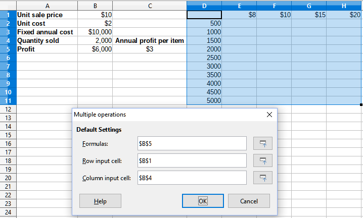
Figure 23: Results of Multiple Operations tool for two variables
Besides scenarios and the Multiple Operations tool, Calc offers a third "what-if" analysis tool called Goal Seek. Typically, you use a formula to calculate a result from given values. However, with Goal Seek, you start with the desired result and work backwards to find the values that produce it. This feature is useful when you know the outcome you want but need to determine how to achieve it or how it might change if you adjust certain conditions.
Note
Only one argument can be altered at a time in a single goal seek. If you need to test multiple arguments, then you must run a separate goal seek on each one.
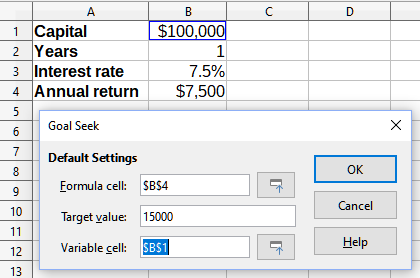
Suppose that we want to calculate the annual interest return for an account. To calculate annual interest (I), we must create a table with values for the capital (C), the interest period length in years (n), and the interest rate (i). The formula is I = C*n*i.
Suppose that the interest rate i = 7.5% (cell B3 of a worksheet) and the period length n = 1 (B2) remain constant. We want to know how much investment capital C is needed to achieve a return of I = $15,000. Assume that our initial capital estimate is C = $100,000 (B1).
To calculate the return:
Enter the return formula (=B1*B2*B3) into B4 and select the cell with the mouse.
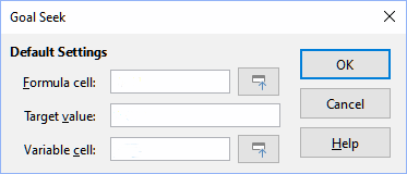
Select Tools > Goal Seek on the Menu bar to open the Goal Seek dialog (Figure 24).
Figure 24: Goal Seek dialog
B4 should already be entered in the Formula cell field. However, if you want to select a different cell, use the associated Shrink / Expand button to minimize the dialog while you select the required cell.
Click on the Variable cell field, then type a reference to cell B1 or select it with the mouse to make the capital the variable in the current Goal Seek.
Enter the desired formula result in the Target value field. In this example, the value is 15000. Figure 25 shows the cells and dialog fields at this point.
Figure 25: Example setup for goal seek
Click OK. A dialog appears informing you that the goal seek was successful (Figure 26).
Figure 26: Goal seek result dialog
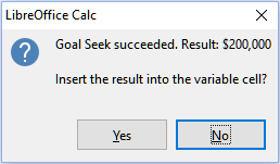
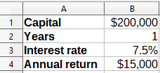
Click Yes to enter the goal value into the variable cell. The result is shown in Figure 27, indicating that a capital requirement of $200,000 is needed to achieve a $15,000 return.
Figure 27: Result of goal seek in worksheet
Note
Not every goal seek problem succeeds in returning a good result. It depends on the formula used, goal value, and initial value. The goal seek algorithm iterates internally several times converging to the goal.
If the goal seek is unsuccessful, Calc displays an information dialog reporting the failure. This dialog offers the choice of inserting the closest value into the variable cell. Press Yes or No as required.
A more elaborate form of goal seek, the Solver, allows you to solve mathematical programming or optimization problems. A mathematical programming problem is concerned with minimizing or maximizing a function subject to a set of constraints. These types of problems occur across various fields, including science, engineering, business, and more. While a comprehensive explanation of mathematical programming is beyond the scope of this guide, readers can explore the topic further on the Mathematical Optimization Wikipedia page. This page offers an overview and links to more in-depth resources.
Calc offers the following selection of solver engines:
DEPS (Differential Evolution & Particle Swarm Optimization) Evolutionary Algorithm.
SCO (Social Cognitive Optimization) Evolutionary Algorithm.
LibreOffice CoinMP Linear Solver.
LibreOffice Linear Solver.
LibreOffice Swarm Non-Linear Solver (experimental).
Caution
As the LibreOffice Swarm Non-Linear Solver is an experimental tool, it may not be supported in future versions of Calc, and we recommend that you do not use it unless you are familiar with non-linear programming concepts.
The DEPS and SCO Evolutionary Algorithms are designed for solving non-linear problems. To use them, you must have a Java runtime environment installed on your computer and enable the Tools > Options > LibreOffice > Advanced > Use a Java runtime environment setting. If available, the DEPS Evolutionary Algorithm is the default solver; otherwise, the LibreOffice CoinMP Linear Solver is used by default.
These options offer flexibility, allowing you to select the algorithm that best fits your specific problem—whether linear or non-linear—and your performance needs. For more detailed information on the available algorithms and their configuration, refer to the Help system.
To use the Solver to solve a mathematical programming problem, you must formulate the problem as follows:
Decision variables – a set of n non-negative variables x1, … , xn,. Decision variables may be real numbers, but generally tend to be integers in many real world problems.
Constraints – a set of linear equalities or inequalities involving the decision variables.
Objective function – a linear expression involving the decision variables.
The goal is usually to find values of the decision variables that satisfy the constraints and maximize or minimize the result of the objective function.
Note
Calc saves solver settings to the ODS file and each tab can have its own model. To support interoperability, the mechanism to save/load solver configurations is compatible with Microsoft Excel.
After setting up the data for the problem in your Calc spreadsheet, select Tools > Solver on the Menu bar to open the Solver dialog (Figure 28).
Note
Depending on the configuration of your computer, a message may be displayed the first time that you select Tools > Solver after starting Calc. The nature of this message will change dependent on the existence of a Java runtime environment (JRE) on your system. If no JRE is detected, the message will simply be a warning to that effect. In the case where a JRE is detected but the Tools > Options > LibreOffice > Advanced > Use a Java runtime environment option is disabled, then the message will include a button to enable that option.
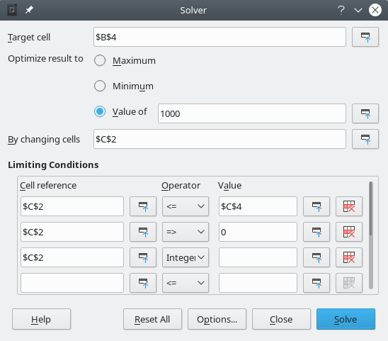
Target cell
Optimize result to
By changing cells
Limiting Conditions
Cell reference – enter a cell reference to a decision variable.
Operator – defines a parameter for a constraint. Available options include <= (less than or equal to), = (equal to), => (greater than or equal to), Integer (values without decimals), and Binary (only 0 or 1).
Value – enter a value or a cell reference to a constraint formula.
Remove button – deletes the currently-defined constraint.
Figure 28: Solver dialog
Tip
Remember that for some of these options, you can minimize the Solver dialog using the associated Shrink / Expand buttons if you need to select cells with the mouse.
After setting up the Solver, click the Solve button to begin adjusting values and calculating results. Depending on the complexity of the problem, this process may take some time. To restart, click the Reset All button, which clears the data entered in the Solver dialog (Figure 28).
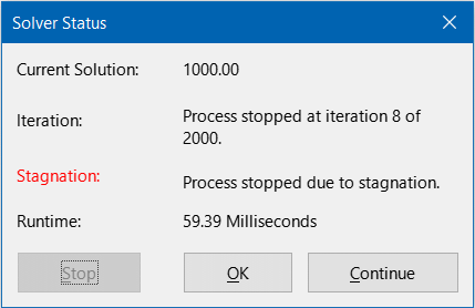
If you are using the DEPS or SCO Evolutionary Algorithm, Calc may occasionally pause the solver engine to display the Solver Status dialog (Figure 29). This dialog provides diagnostic information about the engine’s current progress, which can be useful for advanced users. Click OK to close the dialog and complete the calculations, or click Continue to process one more step, with updated diagnostic information appearing at the next pause. By default, the Solver Status dialog is enabled, but you can disable it by unchecking the Show enhanced solver status option in the Solver Options dialog.
Figure 29: Solver Status dialog
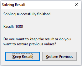
On successful completion, Calc presents a Solving Result dialog (Figure 30). This dialog includes buttons to save (Keep Result) or discard (Restore Previous) your results.
Figure 30: Solving Result dialog
The Options button (Figure 28) opens the Options dialog shown in Figure 31.
Figure 31: Solver Options dialog
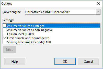
Solver engine
DEPS Evolutionary Algorithm
SCO Evolutionary Algorithm
LibreOffice CoinMP Linear Solver
LibreOffice Linear Solver
LibreOffice Swarm Non-Linear Solver (experimental)
Settings
Suppose that you have $10,000 that you want to invest in two mutual funds for one year. Fund X is a low risk fund with an 8% interest rate and Fund Y is a higher risk fund with a 12% interest rate. How much money should be invested in each fund to earn a total interest of $1,000?
To find the answer using the Solver:
Enter the following labels and data into a worksheet:
Row labels: Fund X, Fund Y, and Total in cells A2, A3, and A4.
Column labels: Interest earned, Amount invested, Interest rate, and Time period in cells B1 thru E1.
Interest rates: 8% and 12% in cells D2 and D3.
Time period: 1 in cells E2 and E3.
Total amount invested: $10000 in cell C4.
Enter an arbitrary value ($0 or leave blank) in cell C2 as the amount invested in Fund X.
Enter the following formulas:
In cell C3, enter the formula =C4–C2 (total amount – amount invested in Fund X) as the amount invested in Fund Y.
In cells B2 and B3, enter the formulas =C2*D2*E2 (B2) and =C3*D3*E3 (B3).
In cell B4, enter the formula =B2+B3 as the total interest earned. Figure 32 shows the worksheet at this point.
Figure 32: Solver example setup
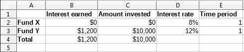
Using the Target cell field, select the cell that contains the target value. In this example, it is B4, which contains the total interest value.
Select Value of and enter 1000 in the field next to it. In this example, the target cell value is 1000 because your target is a total interest earned of $1,000.
Using the By changing cells field, select cell C2 in the sheet. In this example, you need to find the amount invested in Fund X (cell C2).
Enter the following limiting conditions for the variables by using the Cell reference, Operator, and Value fields:
C2 <= C4 – the amount invested in Fund X cannot exceed the total amount available.
C2 => 0 – the amount invested in Fund X cannot be negative.
C2 is an Integer – specified for convenience.
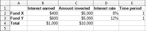
Click Solve. The result is shown in Figure 33.
Figure 33: Solver example result
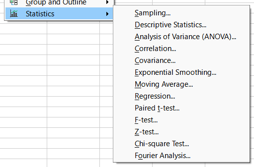
The tools found under Data > Statistics on the Menu bar (Figure 34) are useful for quick and easy statistical analysis of your data.
Figure 34: Statistics menu
These tools are described in the subsections that follow.
Selecting Data > Statistics > Sampling on the menu bar opens the Sampling dialog shown in Figure 34. The Sampling tool creates a target table with data sampled from a source table. It can pick samples randomly or periodically. Sampling is done by rows, with whole rows of the source table copied into rows of the target table.
Figure 35: Sampling dialog
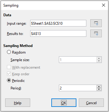
Input range
Results to
Random
Sample size
With replacement
Keep order
Periodic
Period
Tip
The Shrink / Expand buttons in the upper-right corner of the dialog may be used to shrink the dialog using the mouse.
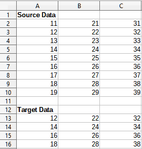
Figure 36 shows the source table (below the Source Data heading) and the corresponding target table (under the Target Data heading), sampled using the settings shown in Figure 35.
Figure 36: Example data for the Sampling tool
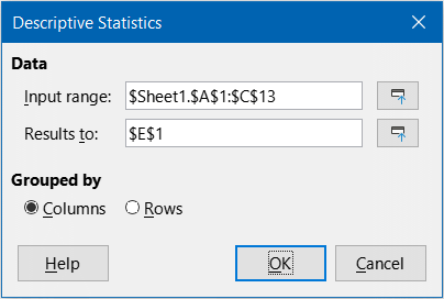
Selecting Data > Statistics > Descriptive Statistics on the Menu bar opens the Descriptive Statistics dialog (Figure 37).Given a set of data, this tool creates a tabular report of the data set’s primary statistical properties, such as information about its central tendency and variability.
Figure 37: Descriptive Statistics dialog
Input range
Results to
Columns / Rows
Figure 38 shows a small data set comprising student examination results in three subjects.
Figure 38: Input data for descriptive statistics analysis
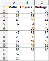
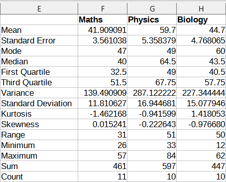
Figure 39 shows the statistics report generated for this input data using the settings shown in Figure 37.
Figure 39: Results from Descriptive Statistics tool
Tip
For more information on descriptive statistics, refer to the corresponding Wikipedia article at https://en.wikipedia.org/wiki/Descriptive_statistics.
Selecting Data > Statistics > Analysis of Variance (ANOVA) on the Menu bar opens the Analysis of Variance (ANOVA) dialog (Figure 40).TThis tool compares the means of two or more groups in a sample.
Input range
Results to
Figure 40: Analysis of Variance (ANOVA) dialog
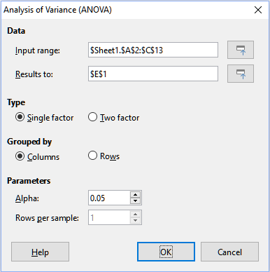
Single factor / Two factor
Columns / Rows
Alpha
Rows per sample
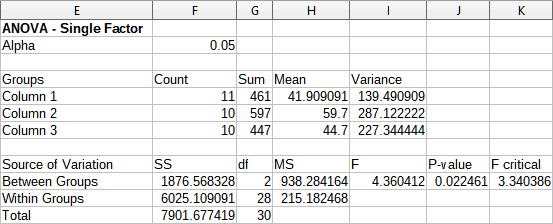
To illustrate how to use this tool, we use the input data set from Figure 38. Figure 41 shows the analysis of variance results generated for this data using the settings shown in Figure 40.
Figure 41: Results from Analysis of Variance (ANOVA) tool
Tip
For more information on analysis of variance, refer to the corresponding Wikipedia article at https://en.wikipedia.org/wiki/Analysis_of_variance.
The Correlation tool measures the relationship between two sets of numeric data and calculates the correlation coefficient. This coefficient, ranging from -1 to +1, indicates the strength and direction of the relationship between the two variables. A coefficient of +1 signifies a perfect positive correlation (the data sets align perfectly), while a coefficient of -1 represents a perfect negative correlation (the data sets are completely inverse). To use this tool, go to Data > Statistics > Correlation in the Menu bar to open the Correlation dialog (Figure 42).
Figure 42: Correlation dialog

Input range
Results to
Columns / Rows
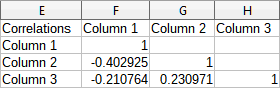
To illustrate how to use this tool, we again use the data set from Figure 38. Figure 43 shows the correlation coefficients generated for this input data using the settings shown in Figure 42.
Figure 43: Correlation results
Tip
For more information on statistical correlation, refer to the corresponding Wikipedia article at https://en.wikipedia.org/wiki/Correlation_and_dependence.
Selecting Data > Statistics > Covariance on the Menu bar opens the Covariance dialog (Figure 44).This tool measures how much two sets of numeric data vary together.
Figure 44: Covariance dialog
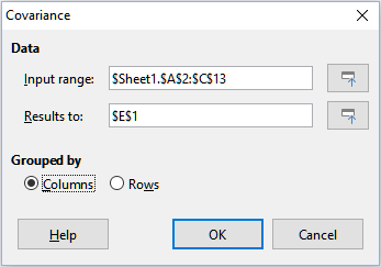
Input range
Results to
Columns / Rows
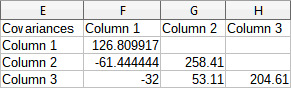
To illustrate how to use this tool, we again use the data set from Figure 38. Figure 45 shows the six covariance values generated for this input data using the settings shown in Figure 44.
Figure 45: Covariance results
Tip
For more information on statistical covariance, refer to the corresponding Wikipedia article at https://en.wikipedia.org/wiki/Covariance.
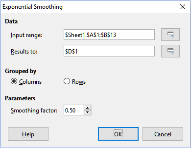
Selecting Data > Statistics > Exponential Smoothing on the Menu bar opens the Exponential Smoothing dialog (Figure 46).This tool filters a data set to produce smoothed results. It is used in domains such as stock market analysis and in sampled measurements.
Figure 46: Exponential Smoothing dialog
Input range
Results to
Columns / Rows
Smoothing factor
To illustrate how to use this tool, we use the data set shown in Figure 47. The table has two time series representing impulse functions at times t=0 and t=2.
Figure 47: Input data set for exponential smoothing example
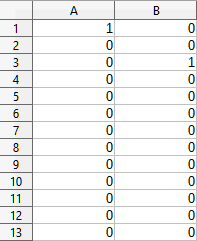
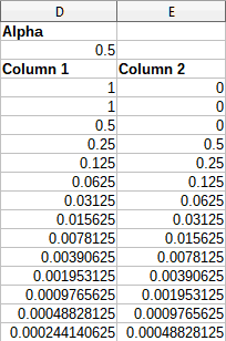
Figure 48 shows the smoothed results for this input data using the settings shown in Figure 46. In the result table, it is possible to change the outcome by varying the Alpha parameter.
Tip
For more information on exponential smoothing, refer to the corresponding Wikipedia article at https://en.wikipedia.org/wiki/Exponential_smoothing.
Figure 48: Results from Exponential Smoothing tool
Selecting Data > Statistics > Moving Average on the Menu bar opens the Moving Average dialog (Figure 49).This tool calculates the moving average of a time series data set.
Figure 49: Moving Average dialog
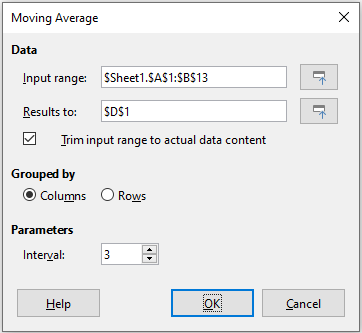
Input range
Results to
Trim input range to actual data content
Columns / Rows
Interval
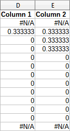
To illustrate how to use this tool, we again use the data set from Figure 47. Figure 50 shows the moving averages calculated for this input data using the settings shown in Figure 49.
Tip
For more information on the moving average, refer to the corresponding Wikipedia article at https://en.wikipedia.org/wiki/Moving_average.
Figure 50: Calculated moving averages
Selecting Data > Statistics > Regression on the Menu bar opens the Regression dialog (Figure 51).This tool performs linear, logarithmic, or power regression analysis of a data set comprising one dependent variable and multiple independent variables.
Figure 51: Regression dialog
Independent variable(s) (X) range
Dependent variable (Y) range
Both X and Y ranges have labels
Results to
Columns / Rows
Linear Regression
Logarithmic Regression
Power Regression
Confidence level
Calculate residuals
Force intercept to be zero
Tip
Calc utilizes the small, otherwise blank area above the Help, OK, and Cancel buttons to provide feedback on erroneous selections on the dialog. For example, the text “Independent variable(s) range is not valid.” appears if a valid cell range has not been entered in the Independent variable(s) (X) range field. In this circumstance, the OK button is disabled until the error is corrected.
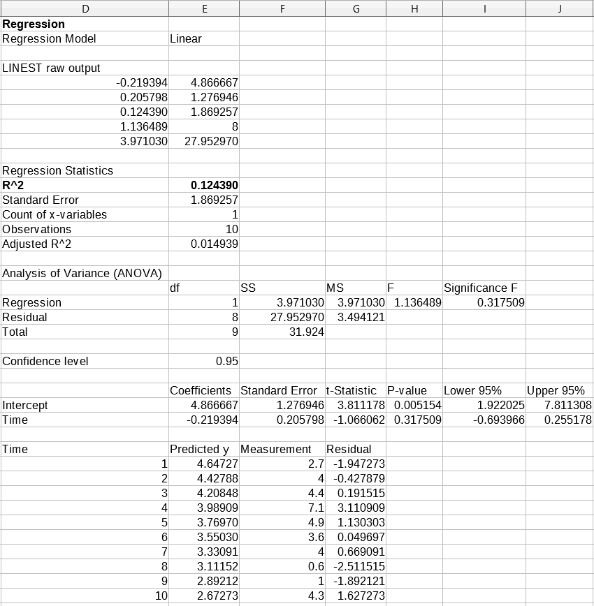
To illustrate how to use this tool, we use the data set shown in Figure 52. This table contains measurements taken at 1 second intervals. Figure 53 shows the regression outputs calculated for this input data using the settings shown in Figure 51.
Tip
For more information on regression analysis, refer to the corresponding Wikipedia article at https://en.wikipedia.org/wiki/Regression_analysis.
Figure 52: Input data set for regression analysis
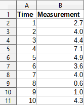
Figure 53: Linear regression outputs
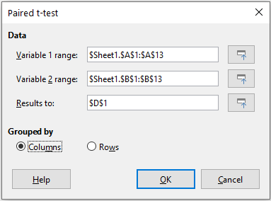
Selecting Data > Statistics > Paired t-test on the Menu bar opens the Paired t-test dialog (Figure 54).This tool compares the population means of two related sample sets and determines the difference between them.
Variable 1 range
Variable 2 range
Results to
Columns / Rows
Figure 54: Paired t-test dialog
To provide an example of using this tool, we make use of the input data set shown in Figure 55. The data sets in columns A and B represent two sets of paired values referred to as Variable 1 and Variable 2.
Figure 55: Input data for paired t-test example
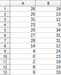
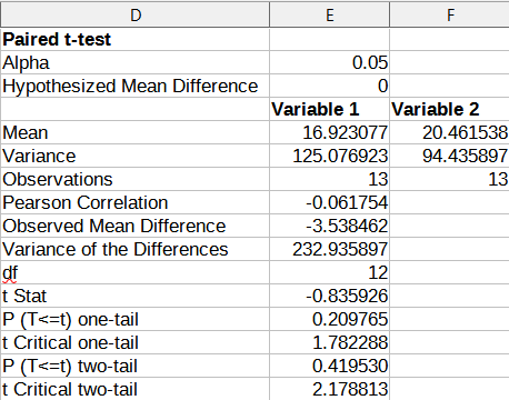
Figure 56 shows the paired t-test results calculated for this input data using the settings shown in Figure 54.
In the resulting table, it is possible to insert different values for Alpha and Hypothesized Mean Difference. The t values (Stat, Critical one-tail, and Critical two-tail) will be updated automatically.
Tip
For more information on paired t-tests, refer to the corresponding Wikipedia article at https://en.wikipedia.org/wiki/Student's_t-test.
Figure 56: Results from Paired t-test tool
Clicking Data > Statistics > F-test on the Menu bar opens the F-test dialog shown in Figure 57 and define the required inputs to the tool.This tool calculates the F-test of two data samples to test the hypothesis that the variance of two populations are equal.
Figure 57: F-test dialog
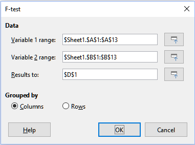
Variable 1 range
Variable 2 range
Results to
Columns / Rows
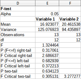
To illustrate how to use this tool, we again use the data set from Figure 55. In this case, the data in columns A and B represent two independent sample sets, referred to as Variable 1 and Variable 2. Figure 58 shows the F-test results calculated for this input data using the settings shown in Figure 57.
In the resulting table, it is possible to insert different values for Alpha. The F Critical values (right-tail, left-tail, and two-tail) will be updated automatically.
Tip
For more information on F-tests, refer to the corresponding Wikipedia article at https://en.wikipedia.org/wiki/F-test.
Figure 58: Results from F-test tool
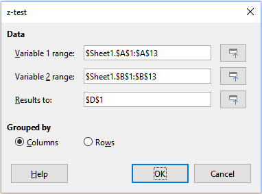
Clicking Data > Statistics > Z-test on the Menu bar opens the Z-test dialog shown in Figure 59 and define the required inputs to the tool.This tool calculates the Z-test of two data samples. It performs a two sample Z-test to test the null hypothesis that there is no difference between the means of the two data sets. The Z-test works better than the Paired t-test tool for large samples (n > 30).
Variable 1 range
Variable 2 range
Results to
Columns / Rows
Figure 59: z-test dialog
To provide an example of using this tool, we again make use of the input data set shown in Figure 55. In this case the data in columns A and B represent two data sets, referred to as Variable 1 and Variable 2. Figure 60 shows the Z-test results calculated for this input data using the settings shown in Figure 59.
Figure 60: Results from Z-test tool
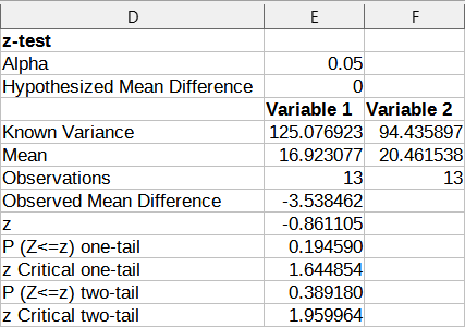
For the Z-test tool to work properly, a known variance for each sample must be inserted in the related cell. In the example shown in Figure 60, the variances (125.076923 and 94.435897) were inserted using the formula =VAR(A1:A13) into cell E5 and the formula =VAR(B1:B13) into cell F5. The subsequent z and P values will be updated automatically.
It is also possible to insert different values for Alpha (cell E2 in the example) and Hypothesized Mean Difference (cell E3 in the example) inputs. As with the known variances changes described above, after changing the Alpha and the Hypothesized Mean Difference, the subsequent z and P values will be updated automatically.
Tip
When analyzing the Z-test results, compare the selected Alpha level with the appropriate calculated P value (depending whether a one-tailed or two-tailed test is required). If the calculated P value is smaller than the Alpha level, the hypothesis (which, in the example given, is that the means of the two data sets are the same) should be rejected.
Tip
For more information on z-tests, refer to the corresponding Wikipedia article at https://en.wikipedia.org/wiki/Z-test.
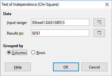
Selecting Data > Statistics > Chi-square Test on the Menu bar opens the Test of Independence (Chi-Square) dialog shown below. This tool calculates the chi-square test of a data sample, which determines how well a set of measured values fit a corresponding set of expected values.
Input range
Results to
Columns / Rows
Figure 61: Test of Independence (Chi-Square) dialog
To provide an example of using this tool, we again make use of the input data set shown in Figure 55. In this case the data in column A is the observed data while the data in column B are the corresponding expected values. Figure 62 shows the chi-square results calculated for this input data using the settings shown in Figure 55.
Figure 62: Results of chi-square test
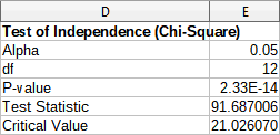
In the resulting table, it is possible to insert different values for Alpha. The Critical Value will be updated automatically.
Tip
For more information on chi-square tests, refer to the corresponding Wikipedia article at https://en.wikipedia.org/wiki/Chi-squared_test.
Selecting Data > Statistics > Fourier Analysis on the Menu bar opens the Fourier Analysis dialog (Figure 63).This tool performs the Fourier analysis of a data set by computing the Discrete Fourier Transform (DFT) of an input array of complex numbers, using Fast Fourier Transform (FFT) algorithms.
Figure 63: Fourier Analysis dialog
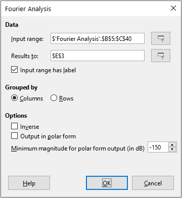
Input range
Results to
Input range has label
Columns / Rows
Inverse
Output in polar form
Minimum magnitude for polar form output
Tip
Calc utilizes the small, otherwise blank area above the Help, OK, and Cancel buttons to provide feedback on erroneous selections on the dialog. For example, the text “Output address is not valid.” appears if a valid cell range has not been entered in the Results to field. In this circumstance, the OK button is disabled until the error is corrected.
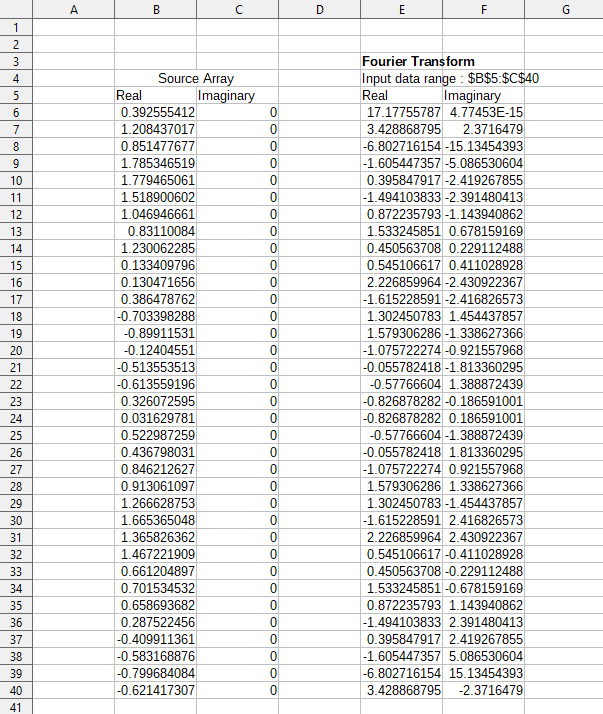
To provide an example of using this tool, we make use of the input data set shown in columns B (real values) and C (imaginary values) of the spreadsheet shown in Figure 64. The data shown in columns E (real values) and F (imaginary values) of the spreadsheet are the Fourier transform results calculated by the tool for this input data, using the settings shown in Figure 63.
Note
The Fourier Analysis tool uses different algorithms depending on the length of the input sequence. If the sequence length is an even power of 2, a radix-2 decimation-in-time FFT algorithm is applied. For sequences of other lengths, Bluestein’s FFT algorithm is used. This detail may be of interest to those with a technical background in algorithms.
Tip
For more information on Fourier analysis, refer to the corresponding Wikipedia article at https://en.wikipedia.org/wiki/Fourier_analysis.
Figure 64: Fourier analysis tool - example input data and results