Copyright
This document is Copyright © 2021 by the LibreOffice Documentation Team. Contributors are listed below. You may distribute it and/or modify it under the terms of either the GNU General Public License (http://www.gnu.org/licenses/gpl.html), version 3 or later, or the Creative Commons Attribution License (http://creativecommons.org/licenses/by/4.0/), version 4.0 or later.
All trademarks within this guide belong to their legitimate owners.
Contributors
|
Felipe Viggiano |
Kees Kriek |
Jean Hollis Weber |
|
Barbara Duprey |
Christian Chenal |
Jean Hollis Weber |
|
Shelagh Manton |
John A Smith |
Peter Schofield |
|
Peter Kupfer |
Andy Brown |
Stephen Buck |
|
Iain Roberts |
Hazel Russman |
Barbara M. Tobias |
|
Jared Kobos |
Dave Barton |
Kees Kriek |
|
Claire Wood |
Steve Fanning |
Leo Moons |
|
Annie Nguyen |
|
|
Feedback
Please direct any comments or suggestions about this document to the Documentation Team’s mailing list: documentation@global.libreoffice.org.
Note
Everything you send to a mailing list, including your email address and any other personal information that is written in the message, is publicly archived and cannot be deleted.
Publication date and software version
Published May 2021. Based on LibreOffice 7.1 Community.
Other versions of LibreOffice may differ in appearance and functionality.
Using LibreOffice on macOS
Some keystrokes and menu items are different on macOS from those used in Windows and Linux. The table below gives some common substitutions for the instructions in this book. For a more detailed list, see the application Help and Appendix A (Keyboard Shortcuts) to this guide.
|
Windows or Linux |
macOS equivalent |
Effect |
|
Tools > Options menu selection |
LibreOffice > Preferences |
Access setup options |
|
Right-click |
Control+click and/or right-click depending on computer setup |
Open a context menu |
|
Ctrl (Control) |
⌘ (Command) |
Used with other keys |
|
Ctrl+Q |
⌘+Q |
Exit / quit LibreOffice |
|
F11 |
⌘+T |
Open the Sidebar’s Styles deck |
Introduction
You can enter data into Calc in several ways: using the keyboard, the Fill tool, and selection lists, as well as dragging and dropping. Calc also provides the ability to enter data into multiple sheets of the same spreadsheet at the same time. After entering data, you can format and display it in various ways.
Entering data
Most data entry in Calc can be done using the keyboard.
Numbers
Click in the cell and type the number using the number keys on either the main keyboard or the numeric keypad.
Negative numbers
To enter a negative number, either type a minus sign in front of the number or enclose the number in parentheses, for example (1234). The result for both methods of entry is the same; for example, –1234.
Leading zeroes
By default, if a number is entered with leading zeroes, for example 01481, Calc will drop the leading zeroes. To retain both the number format and a minimum number of characters in a cell when entering numbers, for example 1234 and 0012, use one of these methods to add leading zeroes.
Method 1
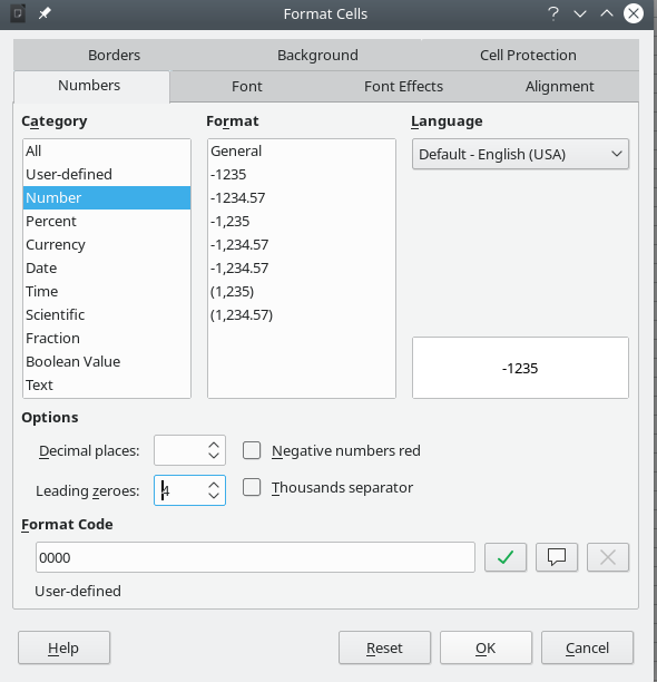
1) With the cell selected, go to Format > Cells on the Menu bar, or right-click on the cell and select Format Cells in the context menu, or use the keyboard shortcut Ctrl+1, to open the Format Cells dialog (Figure 1).
2) Make sure the Numbers tab is selected, then select Number in the Category list.
3) In the Leading zeroes field within the Options area, enter the minimum number of characters required. For example, for four characters, enter 4. Any number less than four characters will then have leading zeroes added, for example 12 becomes 0012.
4) Click OK. The number entered retains its number format and any formula used in the spreadsheet will treat the entry as a number in formula functions.
Tip
To format numbers with only decimal places, but without a leading zero, follow steps and above, then in the Format code box type a . (period or full stop) followed by ? (one or more question marks) to represent the number of decimal places required. For example, for 3 decimal places, type .??? and click OK. Any number with only decimal places will then have no zero before the decimal, for example 0.01856 becomes .019.
Figure 1: Format Cells dialog – Numbers tab
Method 2
1) Select the cell.
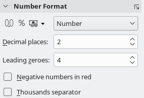
2) On the Sidebar, go to the Properties deck.
3) In the Number Format panel (Figure 2), select Number in the drop-down list, and enter 4 in the Leading zeroes field. Formatting is applied immediately.
Figure 2: Set leading zeroes in Sidebar
Numbers as text
Numbers can also be converted into text using one of the following methods.
Method 1
1) With the cell selected, open the Format Cells dialog (Figure 1).
2) Make sure the Numbers tab is selected, then select Text from the Category list.
3) Click OK. The number is converted to text and, by default, is left-aligned. You can change the formatting and alignment of any text numbers just as you would with normal text.
Method 2
1) Select the cell.
2) On the Sidebar, go to the Properties deck.
3) In the Number Format panel (Figure 2), select Text in the drop-down list. Formatting is applied to the cell immediately.
Tip
If numerical characters do not need to be treated as numbers in calculations (for example when entering zip codes), you can type an apostrophe (') before the number, for example '01481. When you move the cell focus, the apostrophe is removed, the leading zeroes are retained, and the number is converted to left-aligned text.
Text
Click in a cell and type the text. The text is left-aligned by default. Cells can contain several lines of text. If you want to use paragraphs, press Ctrl+Enter to create another paragraph.
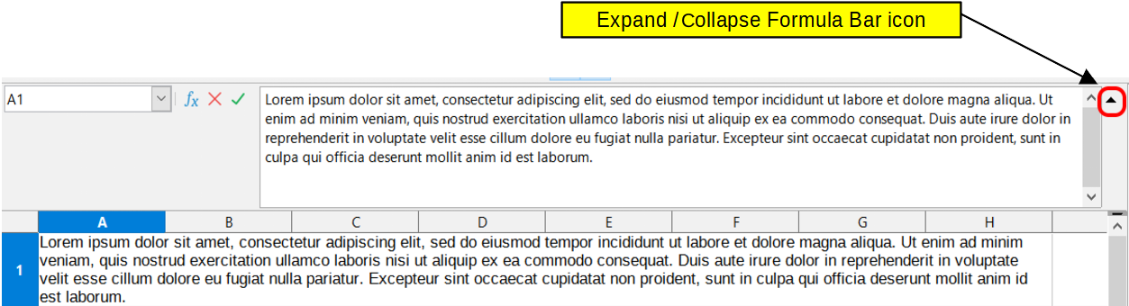
On the Formula Bar, you can extend the Input line if you are entering several lines of text. Click on the Expand / Collapse Formula Bar icon located on the right of the Formula Bar and the Input line becomes multi-line, as shown in Figure 3. You can drag the bottom of the Input line up and down to control its exact height. Click the Expand / Collapse Formula Bar icon again to return the Input line to its default single line height.
Figure 3: Expanded Input line on Formula Bar
Date and time
Select the cell and type the date or time. You can separate the date elements with a slash (/) or a hyphen (–) or use text, for example 10 Oct 2020. The date format automatically changes to the selected format used by Calc.
Note
Tools > Options > Language Settings > Languages > Formats > Date acceptance patterns defines the date patterns that will be recognized by Calc. In addition, every locale accepts input in an ISO 8601 Y-M-D pattern (for example, 2020-07-26).
When you enter a time, separate time elements with colons, for example 10:43:45. The time format automatically changes to the selected format used by Calc.
To change the date or time format used by Calc:
1) With the cell selected, open the Format Cells dialog (Figure 1).
2) Make sure the Numbers tab is selected, then select Date or Time in the Category list.
3) Select the date or time format you want to use from the Format list.
4) Click OK to save the changes and close the dialog.
Note
The date format will be influenced by the system or document language settings.
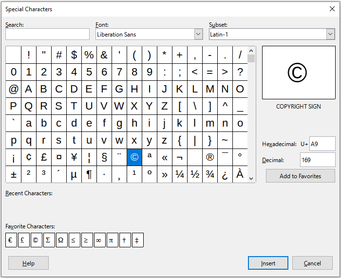
Special characters
A special character is a character not normally found on a standard keyboard; for example, © ¾ æ ç ñ ö ø ¢. To insert a special character:
1) Select a cell and place the cursor in the cell or in the Input line, at the point where you want the character to appear.
2) Go to Insert > Special Character on the Menu bar to open the Special Characters dialog (Figure 4).
3) From the grid of characters, select the required character. The last character selected is shown on the right of the Special Characters dialog along with its numerical code.
4) Any recently inserted characters are shown below the grid of characters and can be selected in the same way as any other character in the dialog.
5) At the bottom of the dialog there is provision for building a small collection of Favorite Characters. To add a new character to the collection, select the required character and click the Add to Favorites button. To remove an existing character from the collection, select the character and click the Remove from Favorites button.
6) Double-click a special character to insert it into the cell, without closing the dialog. Click Insert to insert a selected special character into the cell and close the dialog.
Tip
You can quickly insert one of your recent or favorite special characters by clicking the Insert Special Characters icon on the Standard toolbar and selecting the required character from the drop-down. Click More Characters on this drop-down to open the Special Characters dialog (Figure 4).
Note
Different fonts include different special characters. If you do not find a particular special character you want, try changing the Font and Subset selections.
Figure 4: Special Characters dialog
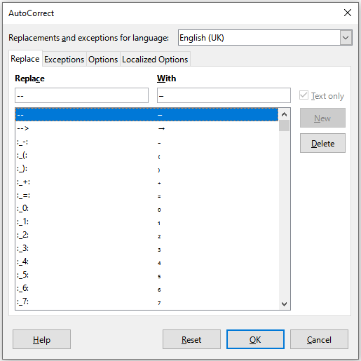
AutoCorrect options
Calc automatically applies many changes during data input using AutoCorrect, unless you have deactivated any AutoCorrect changes. You can undo any AutoCorrect changes by selecting Edit > Undo on the Menu bar, pressing the keyboard shortcut Ctrl+Z, or manually going back to the change and replacing the autocorrection with what you actually want to see.
To change the AutoCorrect options, go to Tools > AutoCorrect Options on the Menu bar to open the AutoCorrect dialog (Figure 5).
-
Replace – edit the replacement table for automatically correcting or replacing words or abbreviations.
-
Exceptions – specify the abbreviations or letter combinations that you do not want corrected automatically.
-
Options – select the options for automatically correcting errors as you type.
-
Localized Options – specify the AutoCorrect options for quotation marks and for options that are specific to the language of the text.
-
Reset – reset modified values back to their previous values.
Figure 5: AutoCorrect dialog
Inserting dashes
Calc provides text shortcuts so that you can quickly insert dashes into a cell and these shortcuts are shown in Table 1.
Table 1: Inserting dashes
|
Text that you type |
Result |
|
A - B (A, space, hyphen, space, B) |
A – B (A, space, en-dash, space, B) |
|
A -- B (A, space, hyphen, hyphen, space, B) |
A – B (A, space, en-dash, space, B) |
|
A--B (A, hyphen, hyphen, B) |
A—B (A, em-dash, B) |
|
A-B (A, hyphen, B) |
A-B (unchanged) |
|
A -B (A, space, hyphen, B) |
A -B (unchanged) |
|
A --B (A, space, hyphen, hyphen, B) |
A –B (A, space, en-dash, B) |
Speeding up data entry
Entering data into a spreadsheet can be very labor-intensive, but Calc provides tools for removing some of the drudgery from input. These tools include drag and drop (to move or copy contents of one location to another using a mouse), an AutoInput tool, the Fill tool, and selection lists.
The Fill tool and selection lists automate input of repetitive material into cells. Calc also has the ability to input information into multiple sheets of the same spreadsheet at the same time.
AutoInput tool
The AutoInput function in Calc automatically completes entries, based on other entries in the same column. The column is scanned up to a maximum of 2000 cells or 200 different strings.
When text is highlighted in a cell, AutoInput can be used as follows:
-
To accept the completion, press Enter or F2, or click the mouse button.
-
To view more completions that start with the same letters, use the key combinations Ctrl+Tab to scroll forward, or Ctrl+Shift+Tab to scroll backward.
-
To see a list of all available AutoInput text items for the current column, use the keyboard combination Alt+↓. See “Selection lists” below for more information.
When typing formulas using characters that match function names, a Help tip will appear listing the available functions that start with matching characters.
AutoInput ignores the case sensitivity of any data you enter. If, for example, you have written “Total” in a cell, you cannot then use AutoInput to enter “total” in another cell of the same column without first deactivating AutoInput or entering “total” manually.
By default, AutoInput is activated in Calc. To turn it off, go to Tools on the Menu bar and deselect AutoInput.
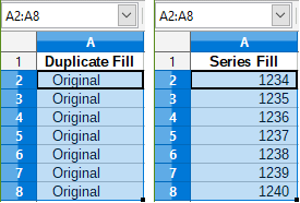
Fill tool
You can use the Fill tool in Calc to duplicate existing content or create a series in a range of cells in the spreadsheet as shown by the examples in Figure 6.
1) Select the cell containing the contents you want to copy or start the series from.
2) Drag the cursor in any direction or hold down the Shift key and click in the last cell you want to fill.
3) Go to Sheet > Fill Cells on the Menu bar and select the direction in which you want to copy or create data (Down, Right, Up, Left, Sheets, Series, or Random Number). A menu option will be grayed out if it is not available.
Figure 6: Examples of using the Fill tool
Tip
You can use the keyboard shortcut Ctrl+D as an alternative to selecting Sheet > Fill Cells > Fill Down on the Menu bar.
Alternatively, you can use a shortcut to fill cells:
1) Select the cell containing the contents you want to copy or start the series from.
2) Move the cursor over the small selection handle in the bottom right corner of the selected cell. The cursor will change shape.
3) Click and drag in the direction you want the cells to be filled, vertical or horizontal. If the original cell contained text, then the text will automatically be copied. If the original cell contained a number or text from a defined list (see “Defining a fill series” below), a series will be created. To duplicate the number or text instead, hold Ctrl while dragging.
Caution
When you are selecting cells so you can use the Fill tool, make sure that none of the cells contain data, except for the cell data you want to use. When you use the Fill tool, any data contained in selected cells is overwritten.
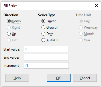
Using a fill series
When you select a series fill from Sheet > Fill Cells > Fill Series on the Menu bar, the Fill Series dialog (Figure 7) opens. Here you can select the type of series you want or create your own list.
-
Direction – determines the direction of series creation.
-
Down – creates a downward series in the selected cell range for the column using the defined increment to the end value.
-
Right – creates a series running from left to right within the selected cell range using the defined increment to the end value.
-
Up – creates an upward series in the selected cell range of the column using the defined increment to the end value.
-
Left – creates a series running from right to left within the selected cell range using the defined increment to the end value.
Figure 7: Fill Series dialog
-
Series Type – defines the series type. These are:
-
Linear – creates a linear number series using the defined increment and end value.
-
Growth – creates a growth series using the defined increment and end value.
-
Date – creates a date series using the defined increment and end date.
-
AutoFill – forms a series directly in the sheet. The AutoFill function takes account of customized lists. For example, by entering January in the first cell, the series is completed using the list defined in Tools > Options > LibreOffice Calc > Sort Lists. AutoFill tries to complete a value series by using a defined pattern. For example, a numerical series using 1,3,5 is automatically completed with 7,9,11,13; a date and time series using 01.01.99 and 15.01.99, is completed using an interval of fourteen days.
-
Time Unit – in this area you specify the desired unit of time. This area is only active if the Date option has been selected in Series Type. The options are:
-
Day – creates a series using seven days.
-
Weekday – creates a series of five day sets.
-
Month – creates a series from the names or abbreviations of the months.
-
Year – creates a series of years.
-
Start value – determines the start value for the series. Use numbers, dates, or times.
-
End value – determines the end value for the series. Use numbers, dates, or times.
-
Increment – determines the value by which the series of the selected type increases by each step. Entries can only be made if the linear, growth, or date series types have been selected.
Defining a fill series
To define your own fill series:
1) Go to Tools > Options > LibreOffice Calc > Sort Lists to open the Sort Lists dialog (Figure 8). This dialog shows any previously defined series in the Lists box on the left and the contents of the highlighted list in the Entries box.
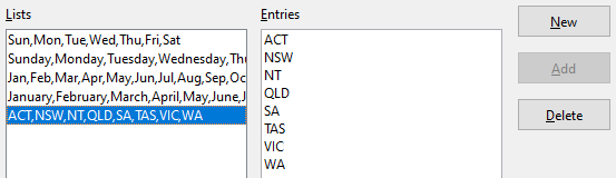
2) Click New and the Entries box is cleared.
3) Type the series for the new list in the Entries box, with one entry per line (Figure 9).
4) Click Add and the new list will now appear in the Lists box.
5) Click OK to save the new list and close the dialog.
Figure 8: Sort Lists dialog
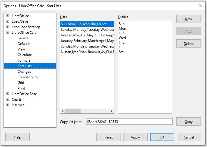
Figure 9: Creating a new sort list
Selection lists
Selection lists are available only for text and are limited to using only text that has already been entered in the same column.
1) Select a blank cell in a column that contains cells with text entries.
2) Right-click and select Selection List in the context menu, or use the keyboard shortcut Alt+↓. A drop-down list appears listing any cell in the same column that either has at least one text character or whose format is defined as text.
3) Click on the text entry you require and it is entered into the selected cell.
Merging and splitting cells
Merging
You can select contiguous cells and merge them into one as follows:
1) Select the range of contiguous cells you want to merge.
2) Go to Format > Merge Cells > Merge Cells or Merge and Center Cells on the Menu bar, or click on the Merge and Center Cells icon on the Formatting toolbar, or right-click on the selected cells and select Merge Cells in the context menu. Using Merge and Center Cells will center align any contents in the cells.
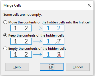
3) If the cells contain any data, the Merge Cells dialog (Figure 10) opens, showing choices for moving or hiding data in the hidden cells.
4) Make your selection and click OK.
Figure 10: Merge choices for non-empty cells
Caution
Merging cells can lead to calculation errors in formulas used in the spreadsheet.
Splitting
You can reverse a merge operation by splitting a cell that was previously created by merging several cells.
1) Select a merged cell.
2) Go to Format > Merge Cells > Split Cells on the Menu bar, or click on the Merge and Center Cells icon on the Formatting toolbar, or right-click and select Split Cells in the context menu.
3) Any data in the cell will remain in the first cell. If the hidden cells did have any contents before the cells were merged, then you may have to manually move the contents to the correct cell.
Sharing content between sheets
You might want to enter the same information in the same cell on multiple sheets, for example to set up standard listings for a group of individuals or organizations. Instead of entering information on each sheet individually, you can enter it in several sheets at the same time.
Figure 11: Select Sheets dialog
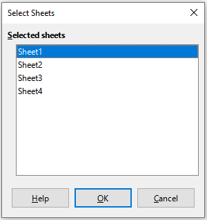
1) Go to Edit > Select > Select Sheets on the Menu bar to open the Select Sheets dialog (Figure 11).
2) Select the individual sheets where you want the information to be repeated.
3) Click OK to select the sheets and the sheet tabs will be highlighted.
4) Enter the information in the cells on the sheet where you want the information to first appear and the information will be repeated in the selected sheets.
5) Deselect the sheets when you have finished entering the information that you want repeated in the sheets.
Tip
You can select sheets with the mouse, as described in the “Selecting sheets” section of Chapter 1, Introduction.
Caution
This technique automatically overwrites, without any warning, any information that is already in the cells on the selected sheets. Make sure you deselect the additional sheets when you have finished entering the information to be repeated before continuing to enter data into the spreadsheet.
Validating cell contents
When creating spreadsheets for other people to use, you may want to make sure they enter data that is valid or appropriate for the cell. You can also use validation in your own work as a guide to entering data that is either complex or rarely used.
Fill series and selection lists can handle some types of data, but are limited to predefined information. For example, a cell may require a date or a whole number with no alphabetic characters or decimal points, or a cell may not be left empty.
Depending on how validation is set up, it can also define the range of contents that can be entered, and provide help messages explaining the content rules set up for the cell and what users should do when they enter invalid content. You can also set the cell to refuse invalid content, accept it with a warning, or start a macro when an error is entered.
Defining validation
To validate any new data entered into a cell:
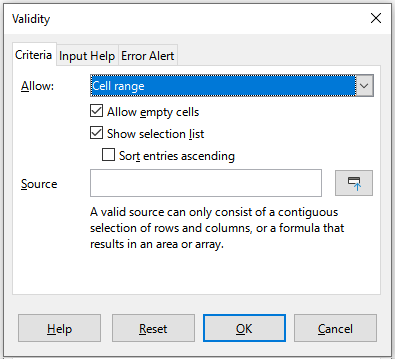
1) Select a cell and go to Data > Validity on the Menu bar to open the Validity dialog (Figure 12).
2) Define the type of contents that can be entered in that cell using the options given on the tabbed pages for Criteria, Input Help, and Error Alert. The options are explained below.
Figure 12: Validity dialog – Criteria tab
Criteria options
Specify the validation rules for the selected cells using the Criteria tab of the Validity dialog as shown in Figure 12. For example, you can define criteria such as numbers between 1 and 10, or texts that are no more than 20 characters.
The options available on the Criteria tab will depend on what has been selected in the Allow drop-down list.
-
Allow – select a validation option for the selected cells from the drop-down list.
-
All values – no limitation.
-
Whole Numbers – only whole numbers allowed.
-
Decimal – all numbers correspond to decimal format.
-
Date – all numbers correspond to date format. The entered values are formatted the next time the dialog is called up.
-
Time – all numbers correspond to time format. The entered values are formatted the next time the dialog is called up.
-
Cell range – allow only values that are given in a cell range. The cell range can be specified explicitly, or as a named database range, or as a named range. The range may consist of one column or one row of cells. If you specify a range of columns and rows, only the first column is used.
-
List – allow only values or strings specified in a list. Strings and values can be mixed. Numbers evaluate to their value, so if you enter the number 1 in the list, the entry 100% is also valid.
-
Text length – allow entries whose length matches the condition on the number of characters that has been set.
-
Custom – allow entries that correspond to a formula entered in the Formula box.
-
Allow empty cells – in conjunction with Tools > Detective > Mark Invalid Data, this defines that blank cells are shown as invalid data (disabled) or not shown (enabled).
-
Show selection list – shows a list of all valid strings or values to select from. The list can be opened either by clicking the down arrow at the right of the cell, or by selecting the cell and pressing Alt+↓.
-
Sort entries ascending – sorts the selection list in ascending order and filters duplicates from the list. If not checked, the order from the data source is taken.
-
Source – enter the cell range that contains the valid values or text.
-
Entries – enter the entries that will be valid values or text strings.
-
Data – select the comparative operator that you want to use from the drop-down list. The available operators depend on what you have selected in the Data drop-down list. For example, if you select valid range, the Minimum and Maximum input boxes replace the Value box.
-
Value – enter the value for the data validation option that you selected in the Data drop-down list.
-
Minimum – enter the minimum value for the data validation option that you selected in the Data drop-down list.
-
Maximum – enter the maximum value for the data validation option that you selected in the Data drop-down list.
-
Formula – enter a formula that can be interpreted as true (non-zero) or false (zero) to provide a custom validation. For example, assuming cell A4 was selected before opening the dialog, you could enter ISEVEN(A4) to indicate that only even values should be entered in cell A4.
Input Help options
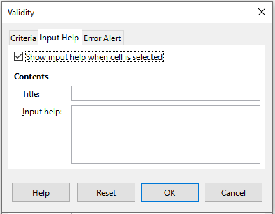
Enter the message to be displayed when the cell or cell range is selected in the spreadsheet (Figure 13).
-
Show input help when cell is selected – displays the message that you enter in the Title and Input help boxes when the cell or cell range is selected in the sheet. If you enter text in the Title and Input help boxes and then deselect this option, the text will not be displayed.
-
Title – enter the title to be displayed when the cell or cell range is selected.
-
Input help – enter the message to be displayed when the cell or cell range is selected.
Figure 13: Validity dialog – Input Help tab
Error Alert options
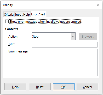
Define the error message that is displayed when invalid data is entered in a cell (Figure 14).
-
Show error message when invalid values are entered – when selected, displays the error message that you enter in the Contents area when invalid data is entered in a cell.
-
Action – select the action that you want to occur when invalid data is entered in a cell.
-
Stop – rejects the invalid entry and displays a dialog that you have to close by clicking OK.
-
Warning and Information – displays a dialog that can be closed by clicking OK or Cancel. The invalid entry is only rejected when you click Cancel.
-
Macro – activates the Browse button to open the Macro Selector dialog where you can select a macro that is executed when invalid data is entered in a cell. The macro is executed after the error message is displayed.
-
Title – enter the title of the macro or the error message that you want to display when invalid data is entered in a cell.
-
Error message – enter the message that you want to display when invalid data is entered in a cell.
Figure 14: Validity dialog – Error Alert tab
Calc Detective
The Detective is a tool within Calc that you can use to locate any cells in a spreadsheet that contain invalid data if the cells are set to accept invalid data with a warning.
1) Go to Tools > Detective > Mark Invalid Data on the Menu bar to locate any cells containing invalid data. The Detective function marks any cells containing invalid data.
2) Correct the data so that it becomes valid.
3) Go to Tools > Detective > Remove All Traces on the Menu bar and any cells that were previously marked as containing invalid data have the invalid data mark removed.
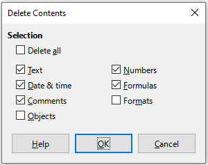
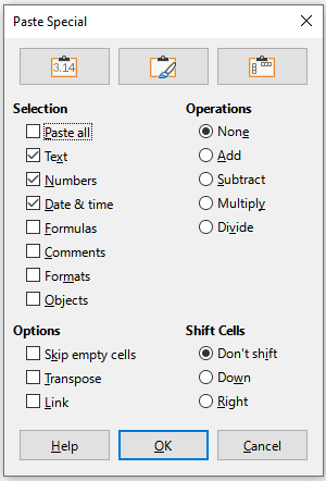
Note
A validity rule is considered part of the format for a cell. If you select Delete all on the Delete Contents dialog (Figure 16), then it is removed. If you want to copy a validity rule with the rest of the cell, use Edit > Paste Special > Paste Special to open the Paste Special dialog (Figure 17), then select Paste all or Formats and click OK.
Editing data
Deleting data
Deleting cell data only
Data can be deleted from a cell without deleting any of the cell formatting. Select a cell or a range of cells and then press the Delete key.
Deleting cells
This option completely deletes selected cells, columns, or rows. The cells below or to the right of the deleted cells will fill the space.
1) Select a cell or a range of cells.
2) Select Sheet > Delete Cells on the Menu bar, or right-click inside the selected cells and choose Delete in the context menu, or press the Ctrl+– keys.
Figure 15: Delete Cells dialog
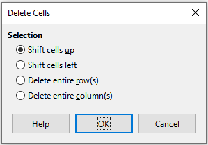
3) The Delete Cells dialog (Figure 15) provides four options to specify how sheets are displayed after deleting cells:
-
Shift cells up. Fills the resulting space with data from the cells underneath.
-
Shift cells left. Fills the resulting space with data from the cells to the right of the deleted cells.
-
Delete entire row(s). After selecting at least one cell, deletes the entire row from the sheet.
-
Delete entire column(s). After selecting at least one cell, deletes the entire column from the sheet.
4) To confirm the selection, click OK.
Note
The selected delete option is stored and reloaded when the dialog is next opened, until LibreOffice is closed. After opening LibreOffice again the delete option contains the default setting.
Deleting data and formatting
Data and cell formatting can be deleted from a cell at the same time. To do this:
1) Select a cell or a range of cells.
2) Select Sheet > Clear Cells on the Menu bar, or right-click inside the selected cells and choose Clear Contents from the context menu, or press the Backspace key.
3) In the Delete Contents dialog (Figure 16), choose any of the options or choose Delete All. Click OK.
Figure 16: Delete Contents dialog
Replacing data
To completely replace data in a cell and insert new data, select the cell and type in the new data. The new data will replace the data already contained in the cell and will retain the original formatting used in the cell.
Alternatively, click in the Input line on the Formula Bar, then double-click on the data to highlight it completely and type the new data.
Editing data
Sometimes it is necessary to edit the contents of a cell without removing all of the data from the cell. For example, changing the phrase “Sales in Qtr. 2” to “Sales rose in Qtr” can be done as follows.
Using the keyboard
1) Click in the cell to select it.
2) Press the F2 key and the cursor is placed at the end of the cell.
3) Press the Backspace key to delete any data up to the point where you want to enter new data.
4) Alternatively, use the keyboard arrow keys to reposition the cursor where you want to start entering the new data in the cell, then press the Delete key or Backspace key to delete any unwanted data before typing the new data.
5) When you have finished editing, press the Enter key to save the changes.
Tip
Each time you select a cell, the contents are displayed in the Input line on the Formula Bar. Using the Input line may be easier when editing data.
Using the mouse
1) Double-click on the cell to select it and place the cursor in the cell for editing.
2) Reposition the cursor to where you want to start editing the data in the cell.
3) Alternatively, single-click to select the cell, then move the cursor to the Input line on the Formula Bar and click at the position where you want to start editing the data in the cell.
4) When you have finished, click away from the cell to deselect it and the editing changes are saved.
Paste Special function
You can use the Paste Special function to paste into another cell selected parts of the data in the original cell or cell range, for example its format or the result of its formula.
Paste Special dialog
1) Select a cell or a cell range.
2) Go to Edit > Copy on the Menu bar, or click the Copy icon on the Standard toolbar, or right-click and select Copy in the context menu, or press Ctrl+C.
3) Select the target cell or cell range.
4) Go to Edit > Paste Special > Paste Special on the Menu bar, or right-click and select Paste Special > Paste Special in the context menu, or use the keyboard shortcut Ctrl+Shift+V, to open the Paste Special dialog (Figure 17).
5) Select the options for Selection, Operations, Options, and Shift Cells. The Paste Special options are explained below.
6) Click OK to paste the data into the target cell or range of cells and close the dialog.
Figure 17: Paste Special dialog
Tip
Instead of steps ) and ) above, you can press one of the three shortcut buttons at the top of the dialog – Values Only, Values & Formats, or Transpose.
Paste Special options
-
Selection – select a format for the clipboard contents that you want to paste.
-
Paste all – pastes all cell contents, comments, formats, and objects into the current document.
-
Text – pastes cells containing text.
-
Numbers – pastes cells containing numbers.
-
Date & time – pastes cells containing date and time values.
-
Formulas – pastes cells containing formulas.
-
Comments – pastes comments that are attached to cells. If you want to add the comments to the existing cell content, select the Add operation.
-
Formats – pastes cell format attributes.
-
Objects – pastes objects contained within the selected cell range. These can be OLE objects, chart objects, or drawing objects.
-
Operations – select the operation to apply when you paste cells into the sheet.
-
None – does not apply an operation when you insert the cell range from the clipboard. The contents of the clipboard will replace existing cell contents.
-
Add – adds the values in the clipboard cells to the values in the target cells. Also, if the clipboard only contains comments, adds the comments to the target cells.
-
Subtract – subtracts the values in the clipboard cells from the values in the target cells.
-
Multiply – multiplies the values in the clipboard cells with the values in the target cells.
-
Divide – divides the values in the target cells by the values in the clipboard cells.
-
Options – sets the paste options for the clipboard contents.
-
Skip empty cells – does not replace target cells with empty cells from the clipboard. If you use this option in conjunction with the Multiply or the Divide operation, the operation is not applied to the target cell of an empty cell in the clipboard. If you select a mathematical operation and deselect Skip empty cells, empty cells in the clipboard are treated as zeroes. For example, if you apply the Multiply operation, the target cells are filled with zeroes.
-
Transpose – pastes the rows of the range in the clipboard as columns of the output range, and the columns of the range in the clipboard as rows.
-
Link – inserts the cell range as a link, so that changes made to the cells in the source file are updated in the target file. To ensure that changes made to empty cells in the source file are updated in the target file, ensure that Paste All is also selected. You can also link sheets within the same spreadsheet. When you link to other files, a DDE link is automatically created. A DDE link is inserted as a matrix formula and can only be modified as a whole.
-
Shift Cells – set the shift options for the target cells when the clipboard content is inserted.
-
Don't shift – replaces target cells with inserted cells.
-
Down – shifts target cells downward when you insert cells from the clipboard.
-
Right – shifts target cells to the right when you insert cells from the clipboard.
Paste Only options
If you only want to copy text, numbers, or formulas to the target cell or cell range:
1) Select the source cell or cell range and copy the data.
2) Select the target cell or cell range.
3) Right-click on the target cell or cell range and select Paste Special in the context menu, then select Text, Number, or Formula.
4) Alternatively, use the Paste Only Text, Paste Only Number, or Paste Only Formula options in the Edit > Paste Special menu on the Menu bar.
Insert cell fields
You can insert a field linked to the date, sheet name, or document name in a cell.
1) Select a cell and double-click to activate edit mode.
2) Right-click and select Insert Field > Date, Time, Sheet Name or Document Title in the context menu.
3) Alternatively use the similar options in the Insert > Field menu on the Menu bar.
Note
The Insert Field > Document Title command inserts the name of the spreadsheet and not the title defined on the Description tab of the Properties dialog for the file.
Tip
The fields are refreshed when the spreadsheet is saved or recalculated when using the Ctrl+Shift+F9 shortcut.
Formatting data
Note
All the settings discussed in this section can also be set as a part of the cell style. See Chapter 4, Using Styles and Templates, for more information.
You can format the data in Calc in several ways, either defined as part of a cell style so that it is automatically applied, or applied manually to the cell. For more control and extra options, select a cell or cell range and use the Format Cells dialog. All of the format options are discussed below.
Multiple lines of text
Multiple lines of text can be entered into a single cell using automatic wrapping or manual line breaks. Each method is useful for different situations.
Automatic wrapping
To automatically wrap multiple lines of text in a cell, use one of the following methods
Method 1
1) Select a cell or cell range.
2) Go to Format > Cells on the Menu bar, or right-click and select Format Cells in the context menu, or press Ctrl+1, to open the Format Cells dialog.
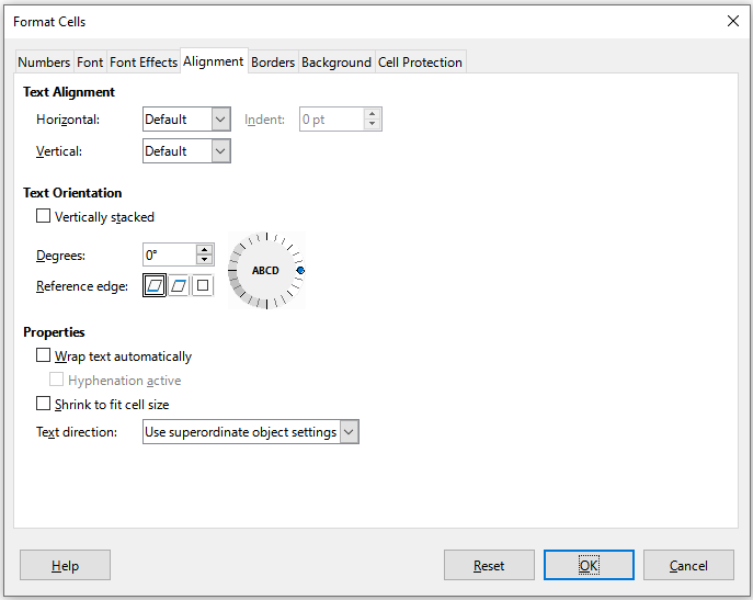
3) Click on the Alignment tab (Figure 18).
4) Under Properties, select Wrap text automatically and click OK.
Figure 18: Format Cells dialog – Alignment tab
Method 2
1) Select the cell.
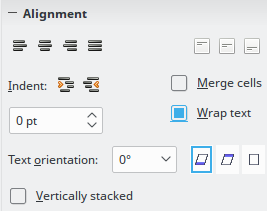
2) On the Properties deck of the Sidebar, open the Alignment panel (Figure 19).
3) Select the Wrap text option to apply the formatting immediately.
Figure 19: Wrap text formatting
Manual line breaks
To insert a manual line break while typing in a cell, press Ctrl+Enter. When editing text, double-click the cell, then reposition the cursor to where you want the line break. In the Input line of the Formula bar, you can also press Shift+Enter.
When a manual line break is entered, the cell row height changes but the cell width may not change and the text may still overlap the end of the cell. You have to change the cell width manually or reposition the line break.
Shrinking text to fit a cell
The font size of the data in a cell can automatically adjust to fit inside cell borders.
1) Select a cell or cell range.
2) Go to Format > Cells on the Menu bar, or right-click and select Format Cells in the context menu, or press Ctrl+1, to open the Format Cells dialog.
3) Click on the Alignment tab (Figure 18).
4) Under Properties, select Shrink to fit cell size and click OK.
Formatting numbers
Several number formats can be applied to cells by using icons on the Formatting toolbar (highlighted in Figure 20). Select the cell, then click the relevant icon to change the number format.
For more control or to select other number formats, use the Numbers tab of the Format Cells dialog (Figure 1):
-
Apply any of the data types in the Category list to the data.
-
Select one of the predefined formats in the Format list.
-
Control the number of decimal places and leading zeroes in Options.
-
Enter a custom format code. This is a very powerful facility that is detailed in the Number Format Codes page of the Help.
-
The Language setting controls the local settings for the different formats such as the date format and currency symbol.
Figure 20: Number icons on Formatting toolbar

Formatting fonts
To select a font and format it for use in a cell:
1) Select a cell or cell range.
2) Click the down arrow on the right of the Font Name box on the Formatting toolbar (highlighted in Figure 21) and select a font in the drop-down list. The font can also be changed using the Font tab on the Format Cells dialog.
3) Click on the down arrow on the right of the Font Size box on the Formatting toolbar and select a font size from the drop-down list. The font size can also be changed using the Font tab on the Format Cells dialog.
4) To change the character format, click on the Bold, Italic, or Underline icons on the Formatting toolbar.
5) To change the paragraph alignment, click on one of the alignment icons (Align Left, Align Center and Align Right). The Format > Align menu also provides these options with addition to the Justified alignment.
Figure 21: Font Name and Size on Formatting toolbar

Note
To specify the language used in the cell, open the Font tab on the Format Cells dialog. Changing language in a cell allows different languages to exist within the same document. For more changes to font characteristics, see “Font effects” below.
Tip
To choose whether to show the font names in their font or in plain text, go to Tools > Options > LibreOffice > View and select or deselect the Show preview of fonts option in the Font Lists section. For more information, see Chapter 14, Setting up and Customizing.
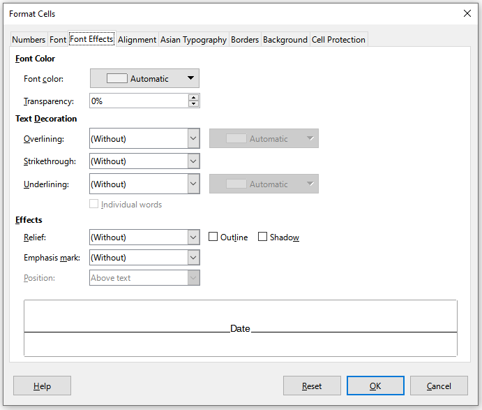
Font effects
1) Select a cell or cell range.
2) Right-click and select Format Cells in the context menu, or go to Format > Cells on the Menu bar, or press Ctrl+1, to open the Format Cells dialog.
3) Click on the Font Effects tab (Figure 22).
4) Select the font effect you want to use from the options available. The options available are described in Chapter 4, Using Styles and Templates.
5) Click OK to apply the font effects and close the dialog.
Any font effect changes are applied to the current selection, or to the entire word that contains the cursor, or to any new text that you type.
Figure 22: Format Cells dialog – Font Effects tab
Text orientation
To change the text direction within a cell, use the Alignment tab on the Format Cells dialog (Figure 18).
1) On the Alignment tab of the Format Cells dialog, select the Reference edge from which to rotate the text as follows:
-
Text Extension From Lower Cell Border – writes the rotated text from the bottom cell edge outwards.
-
Text Extension From Upper Cell Border – writes the rotated text from the top cell edge outwards.
-
Text Extension Inside Cell – writes the rotated text only within the cell.
2) Click on the small indicator at the edge of the text orientation dial and rotate it until you reach the required degrees.
3) Alternatively, enter the number of degrees to rotate the text in the Degrees box.
4) Select Vertically stacked to make the text appear vertically in the cell.
An Asian layout mode checkbox is available on the Alignment tab of the Format Cells dialog when Asian language support is enabled and the text direction is set to vertical. This option aligns Asian characters one below the other in the selected cell(s). If the cell contains more than one line of text, the lines are converted to text columns that are arranged from right to left. Western characters in the converted text are rotated 90 degrees to the right. Asian characters are not rotated.
Using the icons on the Formatting toolbar
The icons on the Formatting toolbar can be used as follows after the cell has been selected:
-
To change the text direction from horizontal (default direction) to vertical, click on the Text direction from top to bottom icon.
-
To change text direction from vertical to horizontal (default), click on the Text direction from left to right icon.
-
To change text direction from left to right, which is the default direction for Western fonts, to a right to left direction used in some fonts, for example Arabic, then click on the Right-To-Left icon. This only works if a font has been used that requires a right to left direction.
-
To change text direction back to the default left to right direction used for Western fonts, click on the Left-To-Right icon.
-
Note
The text direction icons can only be made available if the Asian and Complex text layout options are checked under Tools > Options > Language Settings > Languages > Default Language for Documents. If it is necessary to make the buttons visible, right-click on the toolbar and select Visible Buttons in the context menu, then click on the icon you require and it will be placed on the Formatting toolbar.
Asian typography
If Asian language support is enabled through Tools > Options > Language Settings > Languages > Default Languages for Documents > Asian, an Asian Typography tab is included on the Format Cells dialog (Figure 23). This tab enables setting of typographic options for cells in Asian language documents.
Figure 23: Format Cells dialog - Asian Typography tab
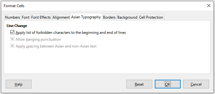
The following options are provided:
-
Apply list of forbidden characters to the beginning and end of lines – prevents the characters in the list of restricted characters from starting or ending a line. The characters are relocated to either the previous or the next line. To edit the list of restricted characters, go to Tools > Options > Language Settings > Asian Layout > First and Last Characters.
-
Allow hanging punctuation – prevents commas and periods from breaking the line. Instead, these characters are added to the end of the line, even in the page margin.
-
Apply spacing between Asian and non-Asian text – inserts a space between ideographic and alphabetic text.
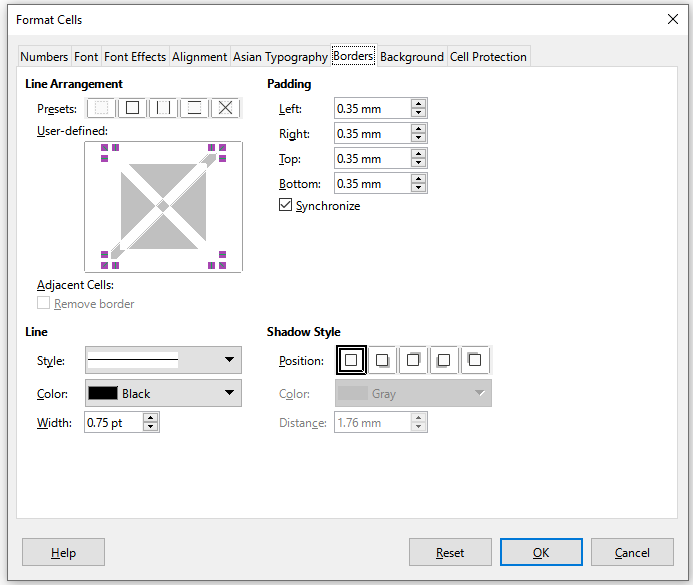
Formatting cell borders
To format the borders of a cell or a group of selected cells, you can use the border icons on the Formatting toolbar to apply the default styles to borders, or the Format Cells dialog for greater control. See Chapter 4, Using Styles and Templates, for more information on the options.
Note
Cell border properties apply only to the selected cells and can only be changed if you are editing those cells. For example, if cell C3 has a top border, that border can only be removed by selecting C3. It cannot be removed in C2, even though it appears to be the bottom border for cell C2.
1) Select a cell or a range of cells.
2) Go to Format > Cells on the Menu bar, or right-click and select Format Cells in the context menu, or press Ctrl+1, to open the Format Cells dialog.
3) On the Borders tab (Figure 24), select the options required.
4) Click OK to close the dialog and save the changes.
Alternatively, use the icons on the Formatting toolbar to apply default styles to borders:
1) Click the Borders icon and select one of the options displayed in the Borders palette.
2) Click the Border Style icon and select one of the line styles from the Border Style palette.
3) Click the Border Color icon to apply the most recently selected color. Click the down arrow to the right of the Border Color icon to select another color from the Border Color palette.
Note
When entering borders with the border icons on the Formatting toolbar, you have two choices: click the required icon to add a border to the present borders or Shift-click to add a border and remove the present borders.
Figure 24: Format Cells dialog – Borders tab
Formatting cell backgrounds
To format the background color for a cell or a group of cells (see Chapter 4, Using Styles and Templates, for more information):
1) Select a cell or a range of cells.
2) Go to Format > Cells on the Menu bar, or right-click and select Format Cells in the context menu, or press Ctrl+1, to open the Format Cells dialog.
3) On the Background tab, click the Color button and select a color from the color palette.
4) Click OK to save the changes and close the dialog.
Alternatively, click on the Background Color icon on the Formatting toolbar to apply the most recently selected color. Click the down arrow to the right of the Background Color icon to select a different color from the Background Color palette.
AutoFormat of cells and sheets
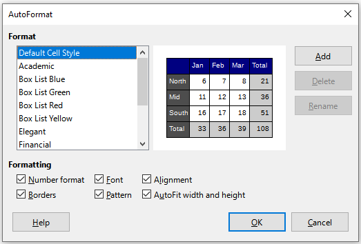
Using AutoFormat
You can use AutoFormat to format a group of cells.
1) Select the cells in at least three columns and rows, including column and row headers, that you want to format.
2) Go to Format > AutoFormat Styles on the Menu bar to open the AutoFormat dialog (Figure 25).
3) Select the type of format and format color in the list.
4) Select the formatting properties to be included in the AutoFormat function.
5) Click OK to apply the changes and close the dialog.
Figure 25: AutoFormat dialog
Defining a new AutoFormat
You can define a new AutoFormat so that it becomes available for use in all spreadsheets.
1) Format the data type, font, font size, cell borders, cell background, and so on for a group of cells.
2) Select a cell range of at least 4x4 cells.
3) Go to Format > AutoFormat Styles to open the AutoFormat dialog. The Add button is now active (if a range smaller than 4x4 cells is selected, the Add button will be unavailable).
4) Click Add.
5) In the Name box of the Add AutoFormat dialog that opens, type a meaningful name for the new format and click OK.
6) The new AutoFormat is now available in the Format list on the AutoFormat dialog. Click OK to close the AutoFormat dialog.
Using themes
Calc comes with a predefined set of formatting themes that you can apply to spreadsheets. It is not possible to add new themes to Calc and the predefined styles cannot be modified. You can modify styles after you apply them to a spreadsheet, but the modified styles are only available for use for that spreadsheet.
To apply a theme to a spreadsheet:
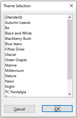
1) Go to Format > Spreadsheet Theme on the Menu bar, or click the Spreadsheet Theme icon on the Tools toolbar, to open the Theme Selection dialog (Figure 26), which lists the available themes for the whole spreadsheet.
2) Select the theme that you want to apply. As soon as you select a theme, the theme styles are applied to the spreadsheet and are immediately visible.
3) Click OK.
Figure 26: Theme Selection dialog
If you wish, you can now use the Styles deck on the Sidebar to modify specific styles. These modifications do not modify the theme; they only change the appearance of the style in the spreadsheet you are creating. For more about modifying styles, see Chapter 4, Using Styles and Templates.
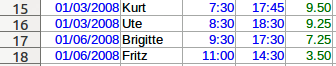
Value highlighting
Value highlighting displays cell contents in different colors depending on the type of content. An example of value highlighting is shown in Figure 27.
-
Text is shown in black.
-
Formulas are shown in green.
-
Numbers (including date and time) are shown in blue.
Figure 27: Example of value highlighting
The value highlighting colors override any colors used in formatting. This color change applies only to the colors seen on a display. When a spreadsheet is printed, the original colors used for formatting are printed.
Go to View > Value Highlighting on the Menu bar, or use the keyboard shortcut Ctrl+F8, to turn the function on or off. When value highlighting is switched off, the original formatting colors are used for display.
You can make value highlighting the default when opening a spreadsheet in Calc, by selecting Tools > Options > LibreOffice Calc > View > Display > Value highlighting. This default mode for value highlighting may not be what you want if you are going to format the cells for printing.
Using conditional formatting
You can set up cell formats to change depending on conditions that you specify. Conditional formatting is used to highlight data that is outside the specifications that you have set. It is recommended not to overuse conditional formatting as this could reduce the impact of data that falls outside those specifications.
See “Conditional formatting example” below for an example of how to use conditional formatting.
Note
Conditional formatting depends upon the use of styles and the AutoCalculate feature must be enabled. If you are not familiar with styles, see Chapter 4, Using Styles and Templates, for more information.
Setting up conditional formatting
1) Ensure that AutoCalculate is enabled: Data > Calculate > AutoCalculate.
2) Select the cells where you want to apply conditional formatting.
3) Go to Format > Conditional > Condition (Figure 28), Color Scale (Figure 29), Data Bar (Figure 30), Icon Set (Figure 31), or Date (Figure 32), on the Menu bar to open the Conditional Formatting dialog. Any conditions already defined are displayed.
4) Click Add to create and define a new condition. Repeat this step as necessary.
5) Select a style from the styles already defined in the Apply Style drop-down list. Repeat this step as necessary.
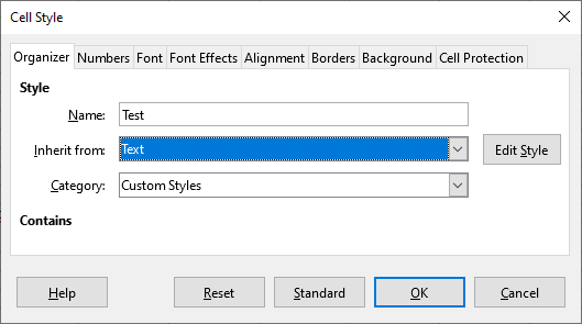
6) Alternatively, select New Style to open the Cell Style dialog (Figure 33) and create a new cell style. Repeat this step as necessary.
7) Click OK to save the conditions and close the dialog. The selected cells are now set to apply a result using conditional formatting.
Figure 28: Conditional Formatting dialog – Condition
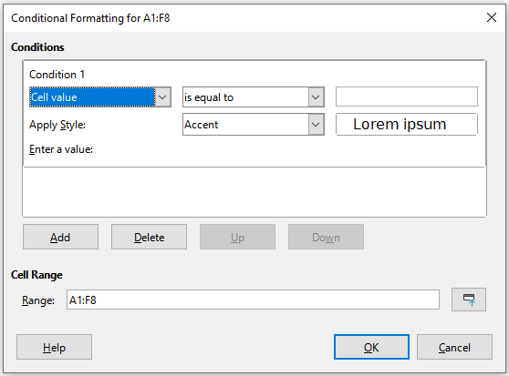
Figure 29: Conditional Formatting dialog – Color Scale
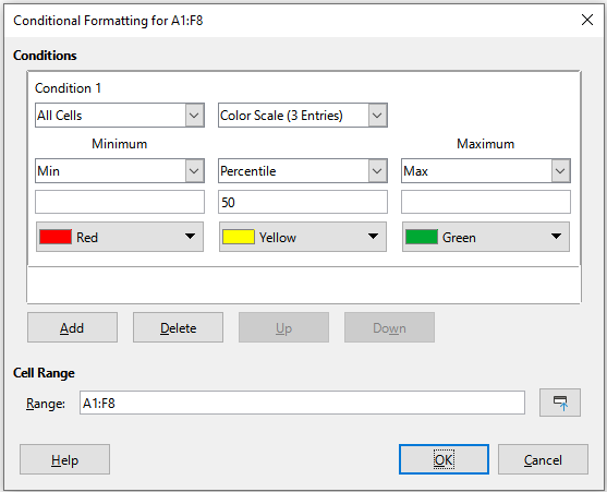
Figure 30: Conditional Formatting dialog – Data Bar
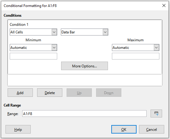
Figure 31: Conditional Formatting dialog – Icon Set
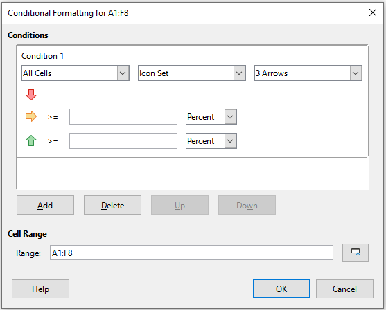
Figure 32: Conditional Formatting dialog - Date
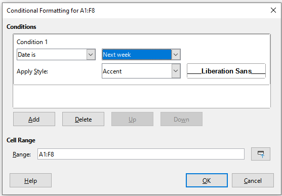
Figure 33: Cell Style dialog
Types of conditional formatting
Condition
Condition is the starting point when using conditional formatting. Here you can define what formats to use to highlight any data in the spreadsheet that falls outside the specifications that you have defined.
Color scale
Use color scale to set the background color of cells depending on the values of the data in those cells. Color scale can only be used when All Cells has been selected for the condition. You can use either two or three colors for the color scale.
Data bar
Data bars provide a graphical representation of data in the spreadsheet. The graphical representation is based on the values of data in a selected range. Click on More Options in the Conditional Formatting dialog to define how the data bars will look. Data bars can only be used when All Cells has been selected for the condition.
Icon set
Icon sets display an icon next to the data in each selected cell to give a visual representation of where the cell data falls within the defined range that you set. The icon sets available include colored arrows, gray arrows, colored flags, colored signs, symbols, bar ratings, and quarters. Icon sets can only be accessed when the Conditional Formatting dialog has been opened and All Cells has been selected for the condition.
Date
Date applies a defined style depending on a data range that you choose in the drop-down menu. Examples include Tomorrow, Last 7 days, This week, Next month, Last year.
Tip
Although each can be accessed using a different option in the Format > Conditional menu of the Menu bar, the five variants of the Conditional Formatting dialog shown in Figures Figure 28 to Figure 32 are not distinct. Once the dialog is open you can create conditions of all types without interacting with the Menu bar. For example, you might create Condition 1 to select a cell style to be used if the cell takes a certain value (Condition 1 is of type “Condition”). You might then press the Add button to create Condition 2 by selecting All Cells in the condition’s upper left drop-down and then selecting Data Bar in the adjacent drop-down (Condition 2 is of type “Data Bar”). You might then press the Add button to create Condition 3 by selecting Date is in the condition’s upper left drop-down (Condition 3 is of type “Date”). In this way you can create many conditions of different types to control the conditional formatting of the selected cells.
Conditional formatting management
To see all the conditional formatting defined in the spreadsheet and any styles used:
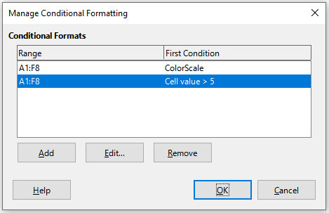
1) Go to Format > Conditional > Manage on the Menu bar to open the Manage Conditional Formatting dialog (Figure 34).
2) Select a range in the Range list and click Edit to redefine the conditional formatting.
3) Select a range in the Range list and click Remove to delete the conditional formatting. The deletion is immediate with no confirmation.
4) Select Add to create a new definition of conditional formatting.
5) Click OK to save the changes and close the dialog.
Figure 34: Manage Conditional Formatting dialog
Copying cell styles
To apply the style used for conditional formatting to other cells later:
1) Click one of the cells that has been assigned conditional formatting and copy the cell to the clipboard.
2) Select the cells that are to receive the same formatting as the copied cell.
3) Go to Edit > Paste Special > Paste Special on the Menu bar, or right-click and select Paste Special > Paste Special in the context menu, or press Crtl+Shift+V, to open the Paste Special dialog (Figure 17).
4) Make sure that only Formats is selected and click OK to paste the conditional formatting into the cell.
Conditional formatting example
One use case for conditional formatting is highlighting the totals that exceed the average value of all totals. If the totals change, the formatting changes correspondingly, without having to apply other styles manually. It is recommended that the Styles deck on the Sidebar is open and visible before proceeding.
Defining conditions
1) Select the cells where you want to apply a conditional style.
2) Go to Format > Conditional > Condition, Color Scale, Data Bar, Icon Set, or Date from the Menu bar to open the Conditional Formatting dialog.
3) Enter the conditions you want to use for conditional formatting.
Generating number values
You may want to give certain values in your tables particular emphasis. For example, in a table of turnovers, you can show all the values above the average in green and all those below the average in red. This is possible with conditional formatting.
1) Create a table in which a few different values occur. For your test, you can create tables with any random numbers. In one of the cells, enter the formula =RAND(), and you will obtain a random number between 0 and 1. If you want integers of between 0 and 50, enter the formula =INT(RAND()*50).
2) Copy the formula to create a row of random numbers.
3) Click the bottom right corner of the selected cell, and drag to the right and downward until the desired cell range is selected.
Defining cell styles
The next step is to apply a cell style to all values that represent above-average turnover and one to cells that are below the average.
1) Right-click in a blank cell and select Format Cells in the context menu to open the Format Cells dialog.
2) Click the Background tab, press the Color button, and select a background color, then click OK.
3) In the Conditional Formatting dialog, select New Style in the Apply Style drop-down list to open the Cell Style dialog.
4) Enter a name of the new style. For this example, name the style Above.
5) Define a second style, click again in a blank cell and proceed as described above. Assign a different background color to the cell and assign a name. For this example, name the style Below.
Calculating average
In our particular example, we are calculating the average of the random values. The result is placed in a cell:
1) Click in a blank cell, for example, J14, and go to Insert > Function on the Menu bar, or click the Function Wizard icon on the Formula Bar, or press Ctrl+F2, to open the Function Wizard dialog.
2) Select AVERAGE in the Functions list.
3) Use the cursor to select all your random numbers.
4) Click OK to close the Function Wizard.
Applying cell styles
Now you can apply the conditional formatting to the sheet:
1) Select all cells containing the random numbers.
2) Go to the Format > Conditional > Condition on the Menu bar to open the Conditional Formatting dialog.
3) Define the condition for each cell as follows: if cell value is less than J14, format with cell style Below OR if cell value is greater than or equal to J14, format with cell style Above.
Hiding and showing data
In Calc you can hide elements so that they are neither visible on a computer display nor printed when a spreadsheet is printed. However, hidden elements can still be selected for copying if you select the elements around them; for example, if column B is hidden, it is copied when you select to copy columns A to C. When you require a hidden element again, you can reverse the process and show the element.
Hiding data
Sheets
Select Sheet > Hide Sheet on the Menu bar, or right-click on the sheet tab for the sheet to be hidden and select Hide Sheet in the context menu. There must always be one sheet that is not hidden.
Rows and columns
1) Select a cell in the row or column you want to hide.
2) Go to Format on the Menu bar and select Rows or Columns.
3) Select Hide from the menu and the row or column can no longer be viewed or printed.
4) Alternatively, right-click on the row or column header and select Hide Rows or Hide Columns in the context menu.
Cells
Hiding individual cells is more complicated. First, you need to define the cells as protected and hidden; then you need to protect the sheet.
1) Select the cells you want to hide.
2) Go to Format > Cells on the Menu bar, or right-click and select Format Cells in the context menu, or press Ctrl+1, to open the Format Cells dialog (Figure 35).
3) Click the Cell Protection tab and select an option for hiding and printing the cells.
4) Click OK to save the changes and close the dialog.
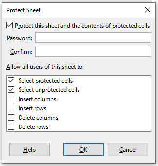
5) Go to Tools > Protect Sheet on the Menu bar, or right-click on the sheet tab and select Protect Sheet in the context menu, to open the Protect Sheet dialog (Figure 36).
6) Select Protect this sheet and the contents of protected cells.
7) Create a password and then confirm the password.
8) Select or deselect the options in the Allow all users of this sheet to area so that users can select protected or unprotected cells.
9) Click OK to save the changes and close the dialog.
Figure 35: Format Cells dialog – Cell Protection tab
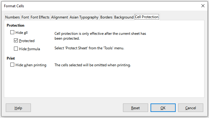
Note
When content in cells is hidden, it is only the content contained in the cells that is hidden and the protected cells cannot be modified. The blank cells remain visible in the spreadsheet.
Figure 36: Protect Sheet dialog
Showing data
Sheets
Select Sheet > Show Sheet on the Menu bar, or right-click on any sheet tab and select Show Sheet in the context menu. Choose which hidden sheets to show from the list on the Show Sheet dialog. If there are no hidden sheets, the Show Sheet option will not appear in the context menu and will be grayed on the Menu bar.
Rows and columns
1) Select the rows or columns on each side of the hidden row or column.
2) Go to Format on the Menu bar and select Rows or Columns. Select Show in the menu and the row or column will be displayed and can be printed.
3) Alternatively, right-click on a row or column header and select Show Rows or Show Columns in the context menu.
Cells
1) Go to Tools > Protect Sheet on the Menu bar, or right-click on the sheet tab and select Protect Sheet in the context menu, to open the Protect Sheet dialog (Figure 36).
2) Enter the password to unprotect the sheet and click OK.
3) Go to Format > Cells on the Menu bar, right-click and select Format Cells in the context menu, or press Ctrl+1, to open the Format Cells dialog (Figure 35).
4) Click the Cell Protection tab and deselect the hide options for the cells. Click OK.
Note
When protecting a sheet using the Protect Sheet dialog, you can leave the password fields blank. In this case, the Protect Sheet dialog is not presented at step ) above and step ) is not necessary.
Group and outline
If you are continually hiding and showing the same cells, you can create an outline of your data and group rows or columns together so that you can collapse a group to hide it or expand a group to show it using a single click.
The basic controls for grouping and outlining show plus (+) or minus (-) signs on the group indicator to show or hide rows or columns. However, if there are groups nested within each other, the basic controls have numbered buttons so you can hide the different levels of nested groups.
Grouping
To group rows or columns:
1) Select the cells you want to group in the spreadsheet.
2) Go to Data > Group and Outline > Group on the Menu bar, or press the F12 key.
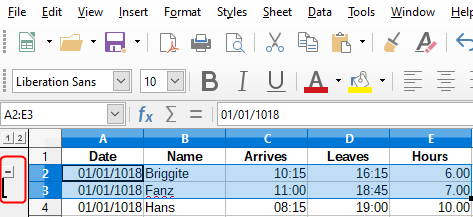
3) On the Group dialog that opens, select either Rows or Columns and click OK. A group indicator appears to the left of any rows grouped or above any columns grouped. Figure 37 shows a group indicator on the left of the first two rows of the spreadsheet showing that they have been grouped.
Figure 37: Group indicator
Hiding details
To hide the details of any group of rows or columns:
1) Click on the minus (–) sign on the group indicator.
2) Alternatively, select a cell within the group and go to Data > Group and Outline > Hide Details on the Menu bar.
3) The rows or columns are hidden and the minus (–) sign becomes a plus (+) sign on the group indicator.
Showing details
To show the details of any hidden groups of rows or columns:
1) Click on the plus (+) sign on the group indicator.
2) Alternatively, select a cell on each side of the hidden group and go to Data > Group and Outline > Show Details on the Menu bar.
3) The hidden rows or columns are displayed and the plus (+) sign becomes a minus (–) sign on the group indicator.
Ungrouping
To ungroup any groups of rows or columns:
1) Make sure the grouped rows or columns are displayed and click on a cell within the group.
2) Go to Data > Group and Outline > Ungroup on the Menu bar, or use the keyboard combination Ctrl+F12.
3) If only rows or only columns are grouped, they are ungrouped. If both rows and columns are grouped, select either Rows or Columns on the Ungroup dialog and click OK.
Caution
Any hidden groups of rows or columns must be displayed. If they are hidden, then the grouped rows or columns are deleted from the spreadsheet.
Note
If there are nested groups, only the last group of rows or columns created is ungrouped.
AutoOutline
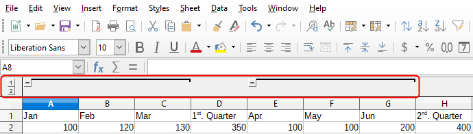
If a selected cell range contains formulas or references, Calc can automatically outline the selection. For example, in Figure 38 the cells for the 1st and 2nd quarters each contain a sum formula for the three cells to their left. If you apply the AutoOutline command, the columns are grouped into two quarters.
To apply the AutoOutline function, go to Data > Group and Outline > AutoOutline on the Menu bar. Calc will then check for cells that contain formulas or references and automatically group the cells as necessary.
Figure 38: Example of AutoOutline
Removing
To remove any cell groups of rows or columns, go to Data > Group and Outline > Remove Outline on the Menu bar and any groups are removed.
For any cell group of rows or columns that are hidden, the grouping is removed from the cells and the cells are displayed in the spreadsheet.
Filtering
A filter is a list of conditions that each entry has to meet to be displayed. Calc provides three types of filters:
-
Standard – specifies the logical conditions to filter the data.
-
AutoFilter – filters data according to a specific value or string. Automatically filters the selected cell range and creates one-row list boxes where you can choose the items that you want to display.
-
Advanced – uses filter criteria from specified cells.
Applying a standard filter
A standard filter is more complex than the AutoFilter. You can set as many as eight conditions as a filter, combining them with the operators AND or OR. Standard filters are mostly useful for numbers, although a few of the conditional operators can also be used for text.
1) Select a cell range in the spreadsheet.
2) Go to Data > More Filters > Standard Filter on the Menu bar to open the Standard Filter dialog (Figure 39).
3) Specify the filter criteria and filtering options that you want to use.
4) Click OK to carry out standard filtering and close the dialog. Any records that match the filter criteria and options that you specified are shown.
Figure 39: Standard Filter dialog
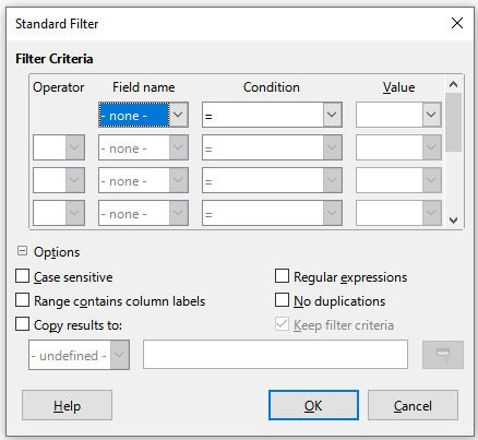
Use the Standard Filter dialog to define the filter conditions to be combined to form the overall filter criteria. Each filter condition is specified by indicating the type of logical operator, the name of a field, a logical condition, and a value.
-
Operator – for the following arguments, you can choose between the logical operators AND and OR. No logical operator is specified for the first filter condition in the list.
-
Field name – specifies the field names from the current table to set them in the argument. You will see the column identifiers if no text is available for the field names.
-
Condition – specifies the comparative operators through which the entries in the Field name and Value fields can be linked.
-
Value – specifies a value to filter the field. The Value list box contains all possible values for the specified Field name. Select a value to be used in the filter, including Empty and Not Empty entries.
-
Case sensitive – distinguishes between uppercase and lowercase letters when filtering the data.
-
Range contains column labels – includes the column labels in the first row of a cell range.
-
Copy results to – select the check box and then select the cell range where you want to display the filter results. You can also select a named range from the list.
-
Regular expressions – select to use regular expressions in the filter definition. If selected, you can use regular expressions in the Value field of the Standard Filter dialog if the Condition field is set to “=” (equal) or “<>” (not equal). For more information about regular expressions, see the section entitled “Regular expressions” in Chapter 1, Introduction.
-
No duplications – excludes duplicate rows from the list of filtered data.
-
Keep filter criteria – select Copy results to and then specify the destination range where you want to display the filtered data. If this box is checked, the destination range remains linked to the source range. You must have defined the source range under Data > Define Range as a database range. You can also reapply the defined filter at any time by clicking into the source range and then going to Data > Refresh Range.
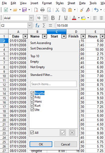
Applying an AutoFilter
An AutoFilter adds a drop-down list to the top row of one or more data columns which lets you select the rows to be displayed. The list includes every unique entry in the selected cells sorted into lexical order (see https://www.dictionary.com/browse/lexical-order for an explanation of lexical order). AutoFilter can be used on multiple sheets without first defining a database range.
1) Click in a cell range on the spreadsheet. If you want to apply multiple AutoFilters to the same sheet, you must first define database ranges, then apply the AutoFilters to the database ranges.
2) Go to Data > AutoFilter on the Menu bar, or click the AutoFilter icon on the Standard toolbar. An arrow button is added to the head of each column in the database range.
3) Click the arrow or small triangle in the column that contains the value or string that you want to set as the filter criteria (shown in Figure 40).
4) Select the value or string that you want to use as the filter criteria. The records that match the filter criteria that you selected are then shown.
Figure 40: AutoFilter example
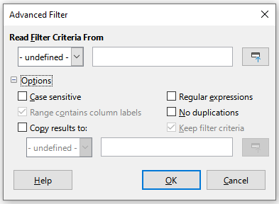
Applying an advanced filter
An advanced filter has a structure similar to a standard filter. The difference is that the advanced filter arguments are not entered in a dialog. Instead, filters can be entered in a blank area of a spreadsheet, then referenced by the filter dialog to apply the filters.
1) Select a cell range in the spreadsheet.
2) Go to Data > More Filters > Advanced Filter on the Menu bar to open the Advanced Filter dialog (Figure 41).
3) In Read Filter Criteria From, select the named range, or enter the cell range that contains the filter criteria that you want to use.
4) Click OK to carry out advanced filtering and close the dialog. Any records that match the filter criteria and options that you specified are shown.
Note
The options for advanced filtering are the same as those used for standard filtering, see “Applying a standard filter” above for more information.
Figure 41: Advanced Filter dialog
For an example of an advanced filter, see the Help page entitled “Filter: Applying Advanced Filters”.
Sorting records
Sorting within Calc arranges the cells in a sheet using the sort criteria that you specify. Several criteria can be used and a sort applies each criteria consecutively. Sorts are useful when you are searching for a particular item and become even more useful after you have filtered data.
Also, sorting is useful when you add new information to a spreadsheet. When a spreadsheet is long, it is usually easier to add new information at the bottom of the sheet, rather than adding rows in their correct place. After you have added information, you can then sort the records to update the spreadsheet.
Sort dialog
To sort cells in a spreadsheet using the Sort dialog:
1) Select the cells, rows, or columns to be sorted.
2) Go to Data > Sort on the Menu bar, or click the Sort icon on the Standard toolbar, to open the Sort dialog.
3) On the Options tab (Figure 42), choose options including whether to sort on rows or columns. See “Sort options” below for details.
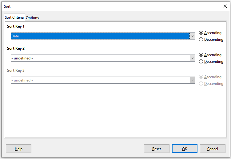
4) On the Sort Criteria tab (Figure 43), select the criteria in the drop-down lists. The selection lists are populated from the selected cells.
5) Select either Ascending order (A-Z, 0-9) or Descending order (Z-A, 9-0).
6) Click OK and the sort is carried out on the spreadsheet.
Note
If any of the cells that you select for sorting are protected and the sheet is protected, then Calc cannot modify those cells and the sort will not be executed. An error message will be displayed to indicate that protected cells cannot be modified. However, it is possible to sort a range containing a row of column labels that are protected, since these are not modified by the sort.
Figure 42: Sort dialog – Options tab
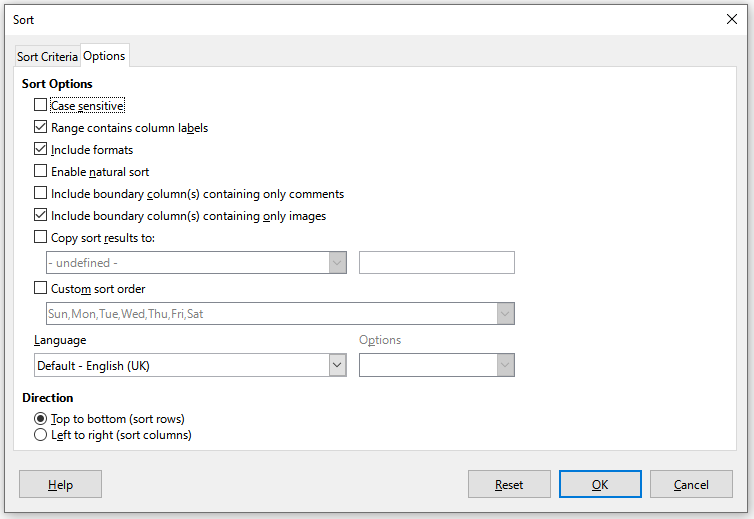
Figure 43: Sort dialog – Sort Criteria tab
Sort options
On the Options tab of the Sort dialog (Figure 42), you can set these options:
-
Case sensitive – sorts first by uppercase letters and then by lowercase letters. For Asian languages, special handling applies.
Note
For Asian languages, select Case sensitive to apply multi-level collation. With multi-level collation, entries are first compared in their primitive forms with their cases and diacritics ignored. If they evaluate as the same, their diacritics are taken into account for the second-level comparison. If they still evaluate as the same, their cases, character widths, and Japanese Kana difference are considered for the third-level comparison.
-
Range contains column/row labels – omits the first column/row in the selection from the sort. The Direction setting at the bottom of the dialog defines the name and function of this check box: if top to bottom, then column labels; if left to right, then row labels.
-
Include formats – preserves the current cell formatting.
-
Enable natural sort – natural sorting is an algorithm that sorts string-prefixed numbers based on the value of the numerical element in each sorted number, instead of the traditional way of sorting them as ordinary strings. For instance, assume you have a series of values such as, A1, A2, A3, A4, A5, A6, ..., A19, A20, A21. When you put these values into a range of cells and run the sort, it will become A1, A11, A12, A13, ..., A19, A2, A20, A21, A3, A4, A5, ..., A9. With natural sorting selected, values such as these are sorted correctly.
-
Include boundary column(s) containing only comments – keeps these cells associated with the cells being sorted.
-
Include boundary column(s) containing only images – keeps these cells associated with the cells being sorted.
-
Copy sort results to – copies the sorted list to the cell range that you specify. Select a named cell range where you want to display the sorted list, or enter a cell range in the input box.
-
Custom sort order – select this option and then select the custom sort order that you want to apply. The available selections are defined as “fill series” in Tools > Options > LibreOffice Calc > Sort Lists. See “Defining a fill series” above.
-
Language – select the language for the sorting rules.
-
Options – select a sorting option for the language. For many languages this selection is grayed out but for some languages options are available. For example, for German the default choice is Alphanumeric, but you can also select the Phone book option to include the umlaut special character in the sorting.
-
Top to bottom (sort rows) – sorts rows by the values in the active columns of the selected range.
-
Left to right (sort columns) – sorts columns by the values in the active rows of the selected range.
Quick sort
If the columns in the spreadsheet have a header with a text format, you can use a quick sort.
1) Select a cell or a cell range to be sorted.
2) Select Data > Sort Ascending or Data > Sort Descending on the Menu bar, or click the Sort Ascending or Sort Descending icon on the Standard toolbar.
Find and replace
Calc has two ways to find text within a document: the Find toolbar and the Find and Replace dialog. The toolbar is quick and easy to use, but its functions are more limited than using the dialog.
Find toolbar
Figure 44: Find toolbar
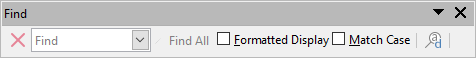
1) Go to View > Toolbars > Find or Edit > Find on the Menu bar, or use the keyboard shortcut Ctrl+F, to open the Find toolbar (Figure 44). By default this toolbar is docked in the lower left of the Calc window. You can undock the toolbar and move it.
2) Type a search term in the Find text box.
3) To refine the search, you can select the Match Case option. For example, if Owner is the search term, selecting Match Case will find Owner but not owner. You can also select the Find All or Formatted Display options.
4) Click the Find Next or Find Previous icon. To find other occurrences of the same term, continue clicking the icon.
Find and Replace dialog
To open the Find and Replace dialog (Figure 45), go to Edit > Find and Replace on the Menu bar, or click the Find and Replace icon on the Standard toolbar or the Find toolbar, or use the keyboard shortcut Ctrl+H.
Finding
1) In the Find and Replace dialog (Figure 45), enter the search criteria in the Find box.
2) Select basic options from those located directly under the Find box.
3) If necessary, click on Other options to increase the number of search filters.
4) Click Find Next to locate the first instance of the search criteria.
5) Click Find Next again to locate the next instance of the search criteria. Repeat as needed.
6) Or, click Find All to locate all cells containing the search criteria. These cells will be highlighted in the spreadsheet. A Search Results dialog will pop up, listing the cell locations.
Replacing
1) In the Find and Replace dialog (Figure 45), enter the search criteria in the Find box.
2) Select basic options from those located directly under the Find box.
3) Enter the replacement contents in the Replace box.
4) If necessary, click on Other options to increase the number of search filters.
5) To step through the cells and choose whether to replace the contents:
6) Click Find Next to locate the first instance of the search criteria.
7) If necessary, click Replace to replace the search criteria with the contents of the Replace box.
8) Repeat as required.
9) Or, to locate and replace all instances of the search criteria without stopping at each one, click Replace All. A Search Results dialog will pop up, listing the affected cells.
Tip
To replace the first instance of the search criteria you can simply press Replace without pressing Find Next first.
Caution
Use Replace All with caution; otherwise, you may end up with some highly embarrassing mistakes. A mistake with Replace All might require a manual, word-by-word search to fix, if it is not discovered in time to undo it.
Figure 45: Find and Replace dialog
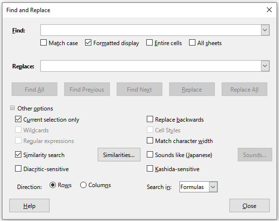
Find and Replace options
The options available to refine your find and replace are as follows:
-
Find – enter the text that you want to search for, or select a previous search in the list.
-
Match case – distinguishes between uppercase and lowercase characters.
-
Formatted display – searches for cell contents in a particular format. For example, if a cell has a currency value, say $123.45 and another has the same contents but default formatting (123.45), then searching for “$123.45” will find the currency cell but not the default-formatted cell.
-
Entire cells – searches for cells with contents that are identical to the search text.
-
All sheets – Searches through all of the sheets in the current spreadsheet file.
-
Replace – enter the replacement text, or select a recent replacement text or style from the list.
-
Current selection only – searches only the selected text or cells.
-
Replace backwards – search starts at the current cursor position and goes backwards to the beginning of the file.
-
Wildcards – select to use wildcards in the search. A wildcard is a special character that represents one or more unspecified characters. Wildcards make text searches more powerful, but often less specific. The following wildcards are available:
-
? (question mark) matches any single character. For example, b?g finds “bag”, “beg”, “big”, “bog”, and “bug”.
-
* (asterisk) matches any sequence of characters, including an empty string. For example, *cast finds “cast”, “forecast”, and “outcast”.
-
~ (tilde) escapes the special meaning of a question mark, asterisk, or tilde character that follows immediately after the tilde character. For example, why~? finds “why?”.
-
Regular expressions – select to use regular expressions in the search. Regular expressions offer the most powerful method of searching for text strings. For more information about regular expressions, see the “Regular expressions” section in Chapter 1, Introduction.
-
Similarity search – find terms that are similar to the Find text. Select this option, and then click the Similarities button to define the similarity options on the Similarity Search dialog.
-
Cell Styles – searches for cell content formatted with the style that you specify. Select this option and then select a style from the Find list. To specify a replacement style, select a style from the Replace list.
-
Diacritic-sensitive – include diacritics and accents in the search.
-
Direction – determines the Rows or Columns order for searching the cells.
-
Search in – select either Formulas, Values, or Comments to search for the characters that you specify in the results of formulas, in values, or in comments.
Other options may appear depending on your language settings on the Tools > Options > Language Settings > Languages page (for example, Match character width, Sounds like (Japanese), Kashida-sensitive). See the Help system for more information about these options.
Note
The Wildcards, Regular expressions, and Similarity search options are mutually exclusive; only one can be selected.
Search Results dialog
After you select Find All on the Find toolbar, or Find All or Replace All on the Find and Replace dialog, Calc’s initial default behavior is to display the Search Results dialog (Figure 46) after it has completed the operation. This dialog summarizes the results. In addition, affected cells are highlighted in the spreadsheet.
The Search Results dialog lists the affected cells and their current content (after any replacement). It also states the number of affected cells. If you deselect the Show this dialog checkbox on the Search Results dialog before pressing the Close button, then the dialog will not be displayed after future uses of Find All or Replace All. The display of the Search Results dialog can also be controlled by enabling or disabling the Tools > Options > LibreOffice Calc > View > Window > Summary on search option.
Figure 46: Search Results dialog