Calc Guide 7.1

Chapter 13
Calc as a Database

Copyright

This document is Copyright © 2021 by the LibreOffice Documentation Team. Contributors are listed below. You may distribute it and/or modify it under the terms of either the GNU General Public License (https://www.gnu.org/licenses/gpl.html), version 3 or later, or the Creative Commons Attribution License (https://creativecommons.org/licenses/by/4.0/), version 4.0 or later.

All trademarks within this guide belong to their legitimate owners.

Contributors

To this edition

Steve Fanning	Kees Kriek	Felipe Viggiano
Jean Hollis Weber

To previous editions

Andrew Pitonyak	Barbara Duprey	Jean Hollis Weber
Simon Brydon	Kees Kriek	Zachary Parliman
Steve Fanning	Leo Moons	Felipe Viggiano

Feedback

Please direct any comments or suggestions about this document to the Documentation Team’s mailing list: documentation@global.libreoffice.org.

Note

Everything you send to a mailing list, including your email address and any other personal information that is written in the message, is publicly archived and cannot be deleted.

Publication date and software version

Published May 2021. Based on LibreOffice 7.1 Community.
Other versions of LibreOffice may differ in appearance and functionality.

Using LibreOffice on macOS

Some keystrokes and menu items are different on macOS from those used in Windows and Linux. The table below gives some common substitutions for the instructions in this book. For a more detailed list, see the application Help and Appendix A (Keyboard Shortcuts) to this guide.

Windows or Linux	macOS equivalent	Effect
Tools > Options menu selection	LibreOffice > Preferences	Access setup options
Right-click	Control+click and/or right-click depending on computer setup	Open a context menu
Ctrl (Control)	⌘ (Command)	Used with other keys
F11	⌘+T	Open the Sidebar’s Styles deck

Introduction

In many everyday scenarios, Calc spreadsheets can be used to aggregate sets of data and to perform analyses on them. As the data in a spreadsheet is laid out in a table view, plainly visible and easily edited or extended, some users may not need the comprehensive relational database facilities provided by the Base component of LibreOffice. For such users, Calc has sufficient functionality to act as a simple yet capable database-like platform. This chapter presents an overview of these capabilities.

For those users who initially choose to manage their data in a Calc spreadsheet and subsequently decide that they need to use a more comprehensive database system, migrating Calc data to Base is straightforward. In the other direction, for Base users who wish to take advantage of some of Calc’s features to analyze or visualize their data, Base can be used for creating linked data ranges in Calc files, for pivot table analysis, or as the basis for charts. See the Base Guide for more information.

Earlier versions of this chapter contained several example LibreOffice Basic macros. These are now available on The Document Foundation’s wiki at https://wiki.documentfoundation.org/Macros/Calc. Much of the macro information on those pages is drawn or adapted from Andrew Pitonyak’s book, OpenOffice.org Macros Explained (OOME) and LibreOffice’s API reference at https://api.libreoffice.org/docs/idl/ref/index.html.

A database primer

In a typical database, related data is organized into tables, which are arranged in a grid-like series of rows and columns similar to a spreadsheet. Each row of a table represents a data record, while each column represents a field within each record. Each cell in a field contains an individual data item or attribute, such as a name, while each record consists of related attributes that correspond to a single entity, like a person. A database table tends to have a fixed number of fields, but can have an indefinite number of records.

While a table may have hundreds or thousands of rows, individual records can be easily found, retrieved, and updated using information requests, called queries, that search for records that meet a specified set of criteria. It is this ease of access that makes a database table more useful than simply filing away information in an unordered spreadsheet.

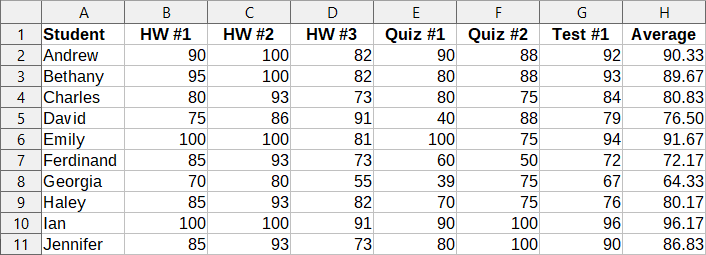
To illustrate this concept of a database table, consider the example of a class grading sheet (Figure 1). In this sheet, each row represents individual students taking the class, while each column contains their names and grades. With this table, you can quickly look up individual students’ grades simply by searching for their names, and you can determine which students are passing the class by filtering out records with failing average scores.

Many modern database management systems are based on the relational database model, in which the data and relationships are represented by a series of inter-related tables. The Base component of LibreOffice is a fully featured relational database management system. Calc does not support the relational database model.

Calc as a database-like program

A Calc sheet is similar to a flat, non-relational database table, and it is possible for a database table to be contained in a Calc sheet. The data can be deeply analyzed using a wide range of tools and functions. It can be sorted, filtered, pivoted, and presented visually in 2-D/3-D charts and graphics. Calc is not a replacement for a fully featured database application but it can be useful for managing data in many small-scale personal or professional contexts.

Associating a range with a name

In order to set up a database table in a Calc sheet, you first need to set up an area for it to occupy. This is necessary since some of Calc’s database-like features depend on accessing or modifying a table’s location. Such an area is represented by a range, which is a contiguous group of one or more cells. To make the range for a table easy to access, you can assign a meaningful name to it. Doing this has four particular benefits:

• Giving a range a name makes it easier to identify, especially if you are working with multiple ranges in a document.

• A named range can be referenced by its name rather than just by its address. For example, if you have a range named Scores, you can simply reference it in a cell with a formula like =SUM(Scores).

• References by name to a named range are automatically updated every time the range’s address is changed. This avoids the need to change individual references every time a range’s location is modified.

• All named ranges can be quickly viewed and accessed through the Navigator, which is opened by selecting View > Navigator on the Menu bar, pressing the F5 key, or clicking the Navigator icon on the Sidebar tab panel.

Two types of named range exist in Calc: database ranges, which store settings for database-like operations, and standard named ranges, which do not.

Named ranges

Technically a named range is a named formula expression and its content is always set as a string. A commonly used type of expression is an absolute cell range like “$Sheet1.$A$1:$E$15”. However, other expression types are possible. For example, the expression “$Sheet1.$A$1:$A$4~$Sheet1.$B$1:$B$4” encompasses two separate cell ranges (the tilde character is a reference concatenation operator). Alternatively a formula expression such as “PI()*B1*B1” might be defined to calculate the area of a circle, given the radius. In the remainder of this section we will be concerned only with named ranges defined as a single rectangular cell range.

A quick way of creating a new named range is to select the relevant cells in your sheet and then simply start typing a name in the Name Box, located at the left of the Formula bar. Notice the “Define Name for Range” tooltip that appears as you type and press the Enter key when you have finished typing.

Named ranges are also created using the Define Name dialog (Figure 2), which is opened either by selecting Sheet > Named Ranges and Expressions > Define on the Menu bar or by clicking the Add button on the Manage Names dialog (Figure 3).

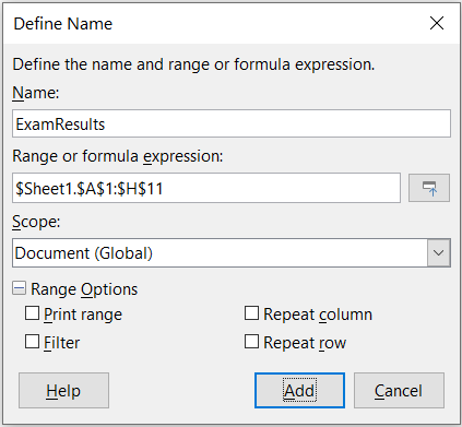
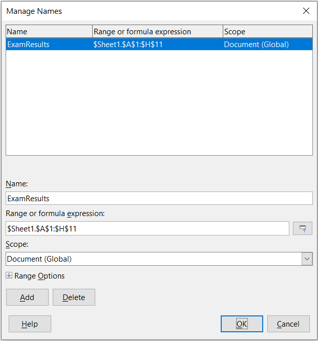
To create a named range, select a range of cells from a sheet, then open the Define Name dialog. Next, give the range a meaningful name, and click on Add to add it to the current document’s list of named ranges. You can then access and modify these ranges using the Manage Names dialog (Figure 3), which is opened by selecting Sheet > Named Ranges and Expressions > Manage on the Menu bar, or pressing Ctrl+F3, or selecting Manage Names in the Name Box located at the left of the Formula bar.

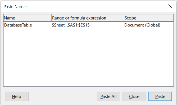
To reduce the typing required when referencing a named range, a Paste Names dialog (Figure 4) can be accessed by selecting Insert > Named Range or Expression or Sheet > Named Ranges and Expressions > Insert on the Menu bar. Select the entry for the relevant named range and click the Paste button to insert the selected named range at the current cursor position.

For more detail about how to create and manage ranges, see Chapter 6, Printing, Exporting, Emailing, and Signing, and Chapter 7, Using Formulas and Functions.

Creating named ranges using row or column headers

With the Create Names tool, which is accessed by selecting Sheet > Named Ranges and Expressions > Create on the Menu bar (Figure 5), you can create multiple named ranges simultaneously from the headers of a table. These headers can be drawn from the table’s borders – top and bottom rows, and left and right columns – and each row or column that corresponds to a header is used to create the named ranges themselves. For example, if you choose to create ranges from headers contained in the top row of a table, each range will be generated from the individual columns that correspond to each header label.

Note

Header cells are not included in the named ranges generated using the Create Names tool. This is because the labels in each of these cells are used to name the ranges.

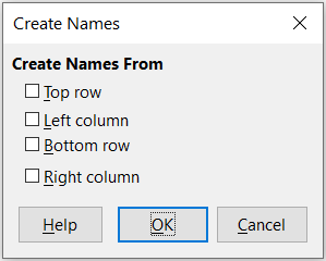
To use the Create Names tool:

1)  In a sheet, select the table from which to create the named ranges. Be sure to include the header rows or columns as part of your selection.

2)  Open the Create Names dialog by selecting Sheet > Named Ranges and Expressions > Create on the Menu bar.

3)  Calc automatically identifies which rows or columns contain headers, and will mark the checkboxes – Top row, Left column, Bottom row, Right column – that apply. However, if you wish to change this selection, you can manually select or deselect any of the boxes at this point.

4)  Click OK to close the dialog and create the new named ranges.

Tip

Avoid giving multiple rows or columns the same label, as the ranges generated from them will likewise share the same name, and can end up being overwritten by Calc.

Database ranges

Although it can be used like a regular named range, a database range is intended to be used like a database table, with each row representing a record and each cell a field within a record. Specifically, a database range differs from a named range in the following ways:

• A database range cannot be a formula expression, only a single rectangular cell range. This range can be formatted as a table, with the first row reserved for headings and the last row for subtotals. Cell formatting can also be preserved for each field in the table.

• Database ranges cannot be referenced relative to a base address within a sheet, which is possible with a named range.

• Database ranges store sorting, filtering, subtotaling, and data import settings in data structures called descriptors, which can be retrieved and accessed using macros. All descriptors of a database range are updated when a database operation is carried out on the cell range of the database range.

• Unlike a named range, a database range can be connected to an external data source, from where you can fetch data into the spreadsheet document.

Database ranges can be created, modified, and deleted using the Define Database Range dialog (Figure 6).

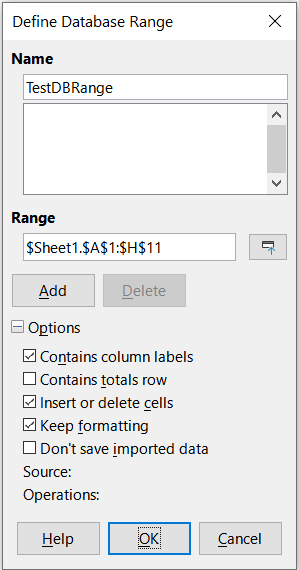
To create a database range:

1)  If you want Calc to automatically determine the full extent of your database table, then select a single cell within its cell area. If you want to explicitly define the extent of the database table, then select all relevant cells.

2)  Open the Define Database Range dialog by selecting Data > Define Range on the Menu bar.

3)  Type a name for the range in the Name field. Only use letters, numbers, and underscores; spaces, hyphens, and other characters are not allowed.

4)  Click on the expand symbol (usually a plus or a triangle) next to the Options label to expand this section and view and select the following options:

• Contains column labels – Denotes whether the top row is reserved for field headings.

• Contains totals row – Denotes whether the bottom row is reserved for totals.

• Insert or delete cells – If active, this option will insert new rows and columns into the database range when new records are added to its source. Only relevant if an external database source is linked to the range. To manually update the database range, use Data > Refresh Range on the Menu bar.

• Keep formatting – Applies the existing cell formats of the first data row to the whole database range.

• Don’t save imported data – If selected, this option only saves a reference to the source database; the contents of the range’s cells are not preserved.

• Source – Displays information about the current database source, if one exists. For example, “Bibliography/biblio”.

• Operations – Denotes what operations (if any) have been applied to the database range. For example, “Sort”, “Filter”, or “Subtotals”.

5)  Click Add to add a range to the database range list under the Name field.

6)  Click OK to close the dialog and save the database range.

To modify an existing database range:

1)  Open the Define Database Range dialog by selecting Data > Define Range on the Menu bar.

2)  Select a range from the range list under the Name field or type its name into the Name field. The Add button will change to Modify at this point.

3)  Make any modifications in the Range field and the Options section.

4)  Click Modify to update the database range.

5)  Click OK to close the dialog and save the modified database range.

To delete an existing database range:

1)  Open the Define Database Range dialog by selecting Data > Define Range on the Menu bar.

2)  Select the range to be deleted from the list in the upper section of the dialog.

3)  Click Delete and then click the Yes button on the confirmation dialog that appears.

4)  Click OK to close the Define Database Range dialog.

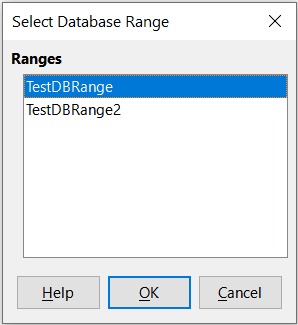
To select an existing database range from the current document, open the Select Database Range dialog by choosing Data > Select Range on the Menu bar (Figure 7). Next, select a range in the Ranges list and click OK. Another way to select an existing database range is using the Navigator deck on the Sidebar. Calc will automatically highlight the range’s position in the sheet in which it is located.

To fetch data from a data source to create a new database range, carry out the following steps:

1)  Open the Data Sources Explorer by selecting View > Data Sources on the Menu bar or pressing Ctrl+Shift+F4.

2)  In the left pane of the Data Sources Explorer, click the expand symbol at the left of the data source name of interest. This action opens the tree to display the tables or queries associated with the data source.

3)  Click on the required table or query to display its constituent data in the right pane of the Data Sources Explorer.

4)  Click on the blank rectangular area at the top left corner of the right pane of the Data Sources Explorer to select all the data in the displayed table or query.

5)  Drag and drop the data to the cell that is to be at the top left corner of the data in your spreadsheet. Search for “drag and drop – data source view” in the Help system for more information about dragging and dropping data from the Data Sources Explorer.

6)  Calc automatically creates a new database range with default parameters, encompassing the cell range of the imported data and with a default name of the form Import1, Import2, etc.

7)  If required, access the Define Database Range dialog (Figure 6) to update settings of the new database range.

Select Data > Refresh Range on the Menu bar to refresh the contents of a database range once the data in the associated data source is updated. The data in the sheet is updated to match the data in the external database. Registering and linking to external database sources are explained in more detail in Chapter 10, Linking Data.

Sorting

Sorting is the process of rearranging data in a range or a sheet according to a specified sort order.

The simplest way to sort a database table based on the contents of a single column is to use the Sort Ascending and Sort Descending tools, as follows:

1)  Select any cell in the column.

2)  To sort in ascending order, select Data > Sort Ascending on the Menu bar or click the Sort Ascending icon on the Standard toolbar. If you have enabled AutoFilters (see next section), you can also select Sort Ascending on the relevant column’s AutoFilter combo box.

3)  To sort in descending order, select Data > Sort Descending on the Menu bar or click the Sort Descending icon on the Standard toolbar. If you have enabled AutoFilters, you can also select Sort Descending on the relevant column’s AutoFilter combo box.

When using the Sort Ascending and Sort Descending tools, Calc automatically identifies the full cell range occupied by your table and sorts the entire area based only on the values in the indicated column. However, it also recognizes the first row as a header row and excludes it from the sort.

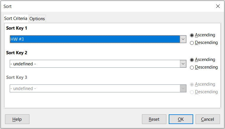
For more complex sorting, use the Sort dialog (Figure 8), which is accessed by selecting Data > Sort on the Menu bar or by clicking the Sort icon on the Standard toolbar. If you select just one cell within the database table before accessing the Sort dialog, then the entire table will be shown as selected when the dialog is displayed.

On the Sort Criteria tab of the dialog, you can specify three levels of sorting. The data is sorted first by the values in the column selected in the Sort Key 1 drop-down, second by the values in the column selected in the Sort Key 2 drop-down, and third by the values in the column selected in the Sort Key 3 drop-down. For example, if you chose Last Name for the first sort key and First Name for the second sort key, the data would primarily be sorted by last name with all rows sharing the same last name sorted by first name.

The Options tab of the Sort dialog provides additional sorting options. For more information about how to use this dialog and its options, see Chapter 2, Entering, Editing, and Formatting Data, and the Help system.

Filtering

A filter is a tool that hides or displays records within a sheet based on a set of filtering criteria. Similar to sorting, filters are useful for narrowing down long lists of data in order to find particular data items. In Calc, three types of filter exist:

• AutoFilters

• Standard filters

• Advanced filters

If you want to remove any filtering applied to your database table, simply select Data > More Filters > Reset Filter on the Menu bar.

Filters are also described in Chapter 2, Entering, Editing, and Formatting Data.

AutoFilter

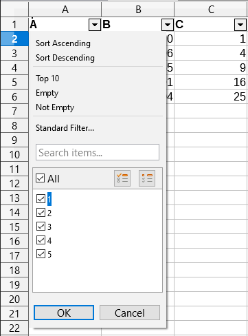
AutoFilters are the most straightforward of the three filter types. They work by providing access to a combo box through a down-arrow button located at the top of one or more data columns (Figure 9). To add AutoFilters to all columns of a database table, click on a cell anywhere within the table area and then select Data > AutoFilter on the Menu bar or click the AutoFilter icon on the Standard toolbar. It is possible to add AutoFilters to individual columns by selecting those columns before choosing Data > AutoFilter or clicking the AutoFilter icon, but this is not normally necessary for a database table. To access the AutoFilter combo box for a column, click on the down-arrow button in the header cell of that column.

To remove AutoFilters from all columns of a database table, click on a cell anywhere within the table area and select Data > AutoFilter on the Menu bar, select Data > More Filters > Hide AutoFilter on the Menu bar, or click the AutoFilter icon on the Standard toolbar. The down-arrow buttons at the tops of columns will disappear.

Tip

Selecting Data > AutoFilter and clicking the AutoFilter icon normally toggle AutoFilters on/off.

Each AutoFilter combo box provides the following options:

• A basic sort can be applied using the Sort Ascending and Sort Descending options.

• Selecting the Top 10 filter causes the ten rows with the largest values to be displayed. More than ten rows may be displayed if there are multiple instances of large values in a column. For example, if there are eleven students with a perfect score of 100, then the filter will display all eleven instances. Similarly, if there are six students with a score of 100 and six other students with a score of 99, then the filter will display twelve instances.

• Selecting Empty hides all non-empty rows that contain a value in the current column. Likewise, selecting Not Empty hides all non-empty rows that lack a value in the current column. Entirely empty rows are ignored but these would not be expected inside a database table.

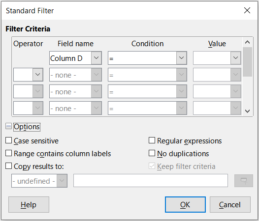
• The Standard Filter option opens the Standard Filter dialog (Figure 10) and automatically sets the current field as the field for the first condition in the dialog.

• Check the All box to display or hide all values in the current column.

• Show only the current item and Hide only the current item shortcut buttons are provided, located adjacent to the All box. In the context of these buttons, the term “current” refers to the item highlighted in the set of check boxes below the buttons (for example the “1” in Figure 9).

• The AutoFilter combo box includes check boxes for each unique value in the current column. If a check box is not ticked, rows of the database table that contain that value in this column are not displayed. Change the filtering status of a particular value by marking or removing the mark from the relevant check box.

Standard filters

Standard filters are more complex than AutoFilters, and allow for up to eight filter conditions. Powerful filters can be set up using regular expressions. Also, unlike AutoFilters, standard filters use a dialog (Figure 10), which is accessed by selecting Data > More Filters > Standard Filter on the Menu bar or the Standard Filter option on an AutoFilter combo box.

For more information on how to use this dialog and its options, see Chapter 2, Entering, Editing, and Formatting Data.

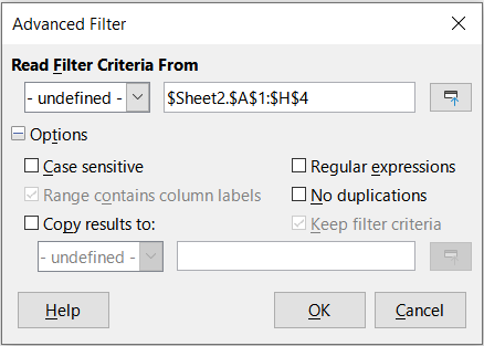
Advanced filters

The criteria for an advanced filter are stored in a sheet rather than entered into a dialog. As a result, you must first set up a cell range that contains the criteria before you use the Advanced Filter dialog (Figure 11).

To set up a criteria range:

1)  Copy the column headings of the range to be filtered to an empty space in a sheet. It does not need to be the same sheet as the one with the source range.

2)  Enter filter criteria underneath the column headings in the criteria range. Each individual criterion in the same row is connected with AND, while the criteria groups from each row are connected with OR. Empty cells are ignored. Up to eight criteria rows may be defined for a filter.

Tip

Although it is possible for the criteria area to contain only the headings for columns with defined filter criteria, for simplicity you may choose to copy all of your database table’s headings to the criteria area.

After creating a criteria range, set up an advanced filter as follows:

1)  Select the cell range that you wish to filter. For a database table you can simply click a cell within the table area and Calc will automatically select the whole table as it opens the dialog at step 2.

2)  Go to Data > More Filters > Advanced Filter on the Menu bar to open the Advanced Filter dialog (Figure 11).

3)  In the Read Filter Criteria From field, enter the address for the criteria range, either by selecting a named range from the drop-down box, typing in a reference, or selecting cells from a sheet. Remember to use the Shrink / Expand button if you need to temporarily minimize the dialog while selecting cells.

4)  Click OK to apply the filter and close the dialog.

Note

For an individual named range, it is possible to tick a Filter checkbox on the Define Name and Manage Names dialogs (Figures Figure 2 and Figure 3 respectively). Only named ranges marked for filtering in this way can be selected in the drop-down box in the Read Filter Criteria From area of the Advanced Filter dialog. Database ranges cannot be selected in the drop-down box.

Advanced filter options are the same as standard filter options, and are described in further detail in Chapter 2, Entering, Editing, and Formatting Data.

Figure 12 demonstrates an example criteria range for the grading sheet example in Figure 1.

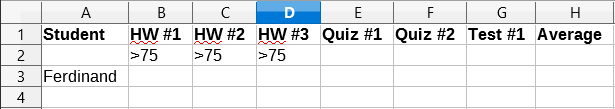
In this range, there are two criteria groups: the first displays the records of students who scored above a 75% in every homework, and the second displays records of any student named “Ferdinand”. Figure 13 displays the result of this filter operation using these criteria.

Useful database-like functions

Database category functions

Overview

The twelve functions in the Database category are intended to help you analyze a simple database that occupies a rectangular spreadsheet area comprising columns and rows, with the data organized as one row for each record. The header cell of each column displays the name of the column and that name usually reflects the contents of each cell in that column.

The functions in the Database category take three arguments as follows:

1)  Database. The cell range of the database.

2)  DatabaseField. The column containing the data to be used in the function’s calculations.

3)  SearchCriteria. The cell range of a separate area of the spreadsheet containing search criteria.

These arguments are described more fully below.

All functions have the same simple concept of operation. The first logical step is to use the specified SearchCriteria to identify the subset of records in the Database that are to be used during subsequent calculations. The second step is to extract the data values and perform the calculations associated with the specific function (average, sum, product, and so on). The values processed are those in the DatabaseField column of the selected records.

Database function arguments

The following argument definitions apply for all functions in the Database category:

Database argument

Database specifies the range of cells occupied by the database table. The first row of the range contains the field names, and subsequent rows are records with corresponding field values.

One way of defining the range of cells is to enter the cell reference for the upper left-hand cell, followed by a colon (:), and then the lower right-hand cell reference. An example might be A1:E10.

The Database argument may also be specified by passing the name of a named range or database range. Using a meaningful name to define the cell range can enhance formula readability and document maintenance. If the name does not match the name of a defined range, Calc reports a #NAME? error.

Other errors that might be reported as a result of an invalid Database argument are #VALUE! and Err:504 (error in parameter list).

DatabaseField argument

DatabaseField specifies the column which the function will use for its calculations after the search criteria have been applied and the data rows have been selected. It is not related to the search criteria.

Specify the DatabaseField argument in any of the following ways:

• By entering a reference to a header cell within the Database area. Alternatively, if the cell has been given a meaningful name as a named range or database range, enter that name. If the name does not match the name of a defined range, Calc reports a #NAME? error. If the name is valid but does not correspond to one cell only, Calc reports Err:504 (error in parameter list).

• By entering a number to specify the column within the Database area, starting with 1. For example, if a Database occupied the cell range D6:H123, then enter 3 to indicate the header cell at F6. Calc expects an integer value that lies between 1 and the number of columns defined within Database and ignores any digits after a decimal point. If the value is less than 1, Calc reports Err:504 (error in parameter list). If the value is greater than the number of columns in Database, Calc reports a #VALUE! error.

• By entering the literal column header name from the first row of the Database range, placing quotation marks around the header name; for example, “Distance to School”. If the string does not match one of the Database area’s column headings, Calc reports Err:504 (error in parameter list). You can also provide a reference to an arbitrary cell (not within the Database and SearchCriteria areas) that contains the required string.

The DatabaseField argument is optional for the DCOUNT and DCOUNTA functions but it is required for the other ten Database functions.

SearchCriteria argument

SearchCriteria specifies the range of cells containing search criteria. Like Database, its first row is also field names, and subsequent rows are conditions for related fields. The Database and SearchCriteria areas need not be adjacent, or even on the same sheet.

One way of defining the range of cells is to enter the cell reference for the upper left-hand cell, followed by a colon (:), and then the lower right-hand cell reference; for example, A13:B14. The cell range may also be specified by passing the name of a defined named range or database range. If the name does not match the name of a defined range, Calc reports a #NAME? error.

Err:504 (error in parameter list) may also be reported as a result of an invalid SearchCriteria argument.

The contents of the SearchCriteria area are described in more detail in the next section.

Defining search criteria

The number of columns occupied by the SearchCriteria area need not be the same as the width of the Database area. All headings that appear in the first row of SearchCriteria must be identical to headings in the first row of Database. However, not all headings in Database need appear in the first row of SearchCriteria, while a heading in Database can appear multiple times in the first row of SearchCriteria.

Search criteria are entered into the cells of the second and subsequent rows of the SearchCriteria area, below the row containing headings. Blank cells within the SearchCriteria area are ignored.

Create criteria in the cells of the SearchCriteria area using the comparison operators <, <=, =, <>, >=, and >. = is assumed if a cell is not empty but does not start with a comparison operator.

If you write several criteria in one row, they are connected by AND. If you write several criteria in different rows, they are connected by OR.

Criteria can be created using wildcards, providing that wildcards have been enabled via the Enable wildcards in formulas option on the Tools > Options > LibreOffice Calc > Calculate dialog. When interoperability with Microsoft Excel is important for your spreadsheet, this option should be enabled.

Even more powerful criteria can be created using regular expressions, providing that regular expressions have been enabled via the Enable regular expressions in formulas option on the Tools > Options > LibreOffice Calc > Calculate dialog.

Tip

When using functions where a search criterion string can be a regular expression, the first attempt is to convert the criterion string to numbers. For example, ".0" will convert to 0.0 and so on. If successful, the match will not be a regular expression match but a numeric match. However, switching to a locale where the decimal separator is not the dot makes the regular expression conversion work. To force the evaluation of the regular expression instead of a numeric expression, use some expression that can not be misread as numeric, such as ".[0]" or ".\0" or "(?i).0".

Another setting that affects how the search criteria are handled is the Search criteria = and <> must apply to whole cells option on the Tools > Options > LibreOffice Calc > Calculate dialog. This option controls whether the search criteria you set for the Database functions must match the whole cell exactly. When interoperability with Microsoft Excel is important for your spreadsheet, this option should be enabled.

Example of Database function use

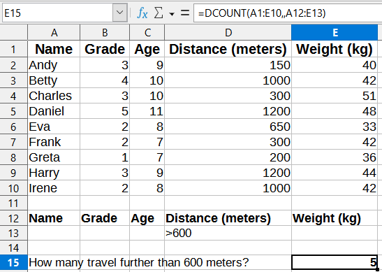
Figure 14 provides a simple example demonstrating how to use one of the functions in the Database category. The formula in the selected cell E15 can be seen in the Formula bar and comprises a call to the DCOUNT function. The arguments of this function call are as follows:

• Database argument. The database table used for this example extends over the cell range A1:E10.

• DatabaseField argument. As the DCOUNT function counts the records that match the criteria without further calculation, it is not necessary to provide a value for this argument, although the relevant argument separators (commas in this case) must be provided.

• SearchCriteria argument. The search criteria area used in this example extends over the cell range A12:E13. The condition in cell D13 (“>600”) will cause DCOUNT to count all records which have a value greater than 600 meters in the Distance (meters) column. In many cases it may be convenient to replicate the column headings of the database table within the search criteria area as shown in Figure 14. However this is not essential and the formula =DCOUNT(A1:E10,,D12:D13) would give exactly the same value of 5.

Many more examples can be found by searching for “database functions” in the Help system, or by visiting the relevant page for each function within the Calc Functions Wiki at https://wiki.documentfoundation.org/Documentation/Calc_Functions.

List of Database functions

Note

Calc will treat dates and logical values (such as TRUE or FALSE) as numeric when calculating with these functions.

DAVERAGE

For all rows (database records) that match the specified search criteria, DAVERAGE calculates the average of the numeric values in the cells (fields) of the specified column. Non-numeric values in those cells are ignored.

Returns a #DIV/0! error if no records match the specified search criteria, or if there are no numeric values in the cells of the specified column for the matching records.

Syntax: DAVERAGE(Database; DatabaseField; SearchCriteria)

DCOUNT

For all rows (database records) that match the specified search criteria, DCOUNT counts the number of cells (fields) of the specified column that contain numeric values. However, if no column is specified, DCOUNT returns the count of all records that match the specified search criteria irrespective of their contents.

Syntax: DCOUNT(Database; [DatabaseField]; SearchCriteria)

DCOUNTA

For all rows (database records) that match the specified search criteria, DCOUNTA counts the number of cells (fields) of the specified column that are not blank. Blank cells of the specified column are not counted. However, if no column is specified, DCOUNTA returns the count of all records that match the specified search criteria irrespective of their contents.

Syntax: DCOUNTA(Database; [DatabaseField]; SearchCriteria)

DGET

For the single row (database record) that matches the specified search criteria, DGET returns the contents of the cell (field) of the specified column.

Calc reports Err:502 (invalid argument) if multiple matches are found, or a #VALUE! error (wrong data type) if no matches are found. A #VALUE! error is also reported if a single match is found but the relevant cell is empty.

Syntax: DGET(Database; DatabaseField; SearchCriteria)

DMAX

For all rows (database records) that match the specified search criteria, DMAX calculates the maximum value across the cells (fields) of the specified column that contain numeric values. Blank cells or cells containing non-numeric characters are not included.

Returns 0 if no matches are found, or if there are no non-zero numeric values in the cells of the specified column for the matching records.

Syntax: DMAX(Database; DatabaseField; SearchCriteria)

DMIN

For all rows (database records) that match the specified search criteria, DMIN calculates the minimum value across the cells (fields) of the specified column that contain numeric values. Blank cells or cells containing non-numeric characters are not included.

Returns 0 if no matches are found, or if there are no non-zero numeric values in the cells of the specified column for the matching records.

Syntax: DMIN(Database; DatabaseField; SearchCriteria)

DPRODUCT

For all rows (database records) that match the specified search criteria, DPRODUCT calculates the product of all numeric values in the cells (fields) of the specified column. Blank cells or cells containing non-numeric characters are not included.

Returns 0 if no matches are found, or if there are no numeric values in the cells of the specified column for the matching records.

Syntax: DPRODUCT(Database; DatabaseField; SearchCriteria)

DSTDEV

For all rows (database records) that match the specified search criteria, DSTDEV calculates the sample standard deviation based on the numeric values in the cells (fields) of the specified column. Non-numeric values are ignored.

Returns a #NUM! error if exactly one record matches the specified search criteria, or if there is only one numeric value in the cells of the specified column for the matching records.

Returns 0 if no matches are found, or if there are no numeric values in the cells of the specified column for the matching records.

Syntax: DSTDEV(Database; DatabaseField; SearchCriteria)

DSTDEVP

For all rows (database records) that match the specified search criteria, DSTDEVP calculates the population standard deviation based on the numeric values in the cells (fields) of the specified column. Non-numeric values are ignored.

Returns a #NUM! error if no records match the specified search criteria, or if there are no numeric values in the cells of the specified column for the matching records.

Syntax: DSTDEVP(Database; DatabaseField; SearchCriteria)

DSUM

For all rows (database records) that match the specified search criteria, DSUM calculates the sum of all numeric values in the cells (fields) of the specified column. Blank cells or cells containing non-numeric characters are not included.

Returns 0 if no matches are found, or if there are no numeric values in the cells of the specified column for the matching records.

Syntax: DSUM(Database; DatabaseField; SearchCriteria)

DVAR

For all rows (database records) that match the specified search criteria, DVAR calculates the sample variance based on the numeric values in the cells (fields) of the specified column. Non-numeric values are ignored.

Returns a #NUM! error if exactly one record matches the specified search criteria, or if there is only one numeric value in the cells of the specified column for the matching records.

Returns 0 if no matches are found, or if there are no numeric values in the cells of the specified column for the matching records.

Syntax: DVAR(Database; DatabaseField; SearchCriteria)

DVARP

For all rows (database records) that match the specified search criteria, DVARP calculates the population variation based on the numeric values in the cells (fields) of the specified column. Non-numeric values are ignored.

Returns a #NUM! error if no records match the specified search criteria, or if there are no numeric values in the cells of the specified column for the matching records.

Syntax: DVARP(Database; DatabaseField; SearchCriteria)

Other database-like functions

Calc includes over 500 functions to help you analyze and reference data. Some of these functions are intended for use with tabular data (such as HLOOKUP and VLOOKUP), while others can be used in any context. This section provides a list of some of the functions that may be useful if you intend to utilize tables in Calc for your database. Many will be familiar as typical spreadsheet functions used in other contexts, while some may be less frequently used but are particularly helpful with database tables.

Further reference material for all Calc’s functions can be found in the Help system and in the Calc Functions area of the The Document Foundation’s wiki, at https://wiki.documentfoundation.org/Documentation/Calc_Functions.

Function	Category	Description
AGGREGATE	Mathematical	Returns an overall result calculated by applying a selected aggregation function to the specified data. Nineteen selectable aggregation functions are available, including average, count, large, maximum, median, minimum, mode, percentile, product, quartile, small, standard deviation, sum, and variance.
AVERAGE	Statistical	Returns the arithmetic mean of the specified data, ignoring empty cells and cells that contain text.
AVERAGEA	Statistical	Returns the arithmetic mean of the specified data, ignoring empty cells but assigning the value 0 to any cell that contains text.
AVERAGEIF	Statistical	Returns the arithmetic mean of all cells in a range that satisfy a given criterion.
AVERAGEIFS	Statistical	Returns the arithmetic mean of all cells in a range that satisfy multiple criteria in multiple ranges.
CHOOSE	Spreadsheet	Returns one value from the specified data, selected according to the index passed as an argument.
COUNT	Statistical	Returns a count of the numeric values in the specified data, ignoring empty cells and cells that contain text.
COUNTA	Statistical	Returns a count of the numeric and text values in the specified data, ignoring empty cells.
COUNTBLANK	Statistical	Returns the number of empty cells in the specified data.
COUNTIF	Statistical	Returns the number of cells in a range that satisfy a given criterion.
COUNTIFS	Statistical	Returns the number of cells that satisfy multiple criteria in multiple ranges.
HLOOKUP	Spreadsheet	Searches for a specified value in the first row of a table (often a column heading) and returns a value retrieved from the same column but a different row. HLOOKUP stands for horizontal lookup.
INDEX	Spreadsheet	Returns the contents of one cell in a table. The position of that cell is specified by row and column offsets. Can also be used in an array formula context to retrieve data from multiple cells.
INDIRECT	Spreadsheet	Returns a valid reference constructed from a supplied string representation of the reference. This function is powerful because it enables a user to create dynamic references.
LOOKUP	Spreadsheet	Searches for a specified value in a single row or column and returns a value from the same position in a second row or column. It is not necessary for the search and result areas to be adjacent.
MATCH	Spreadsheet	Returns the relative position of a search item in a single row or column range.
MAX	Statistical	Returns the maximum value in the specified data, ignoring empty cells and cells that contain text.
MAXA	Statistical	Returns the maximum value in the specified data, ignoring empty cells but assigning the value 0 to any cell that contains text.
MAXIFS	Statistical	Returns the maximum value of all cells in a range that satisfy multiple criteria in multiple ranges.
MEDIAN	Statistical	Returns the median value of the specified data. The median of a finite list of numbers is the "middle" number, when those numbers are listed in order from smallest to greatest.
MIN	Statistical	Returns the minimum value in the specified data, ignoring empty cells and cells that contain text.
MINA	Statistical	Returns the minimum value in the specified data, ignoring empty cells but assigning the value 0 to any cell that contains text.
MINIFS	Statistical	Returns the minimum value of all cells in a range that satisfy multiple criteria in multiple ranges.
MODE MODE.SNGL	Statistical	Returns the mode value of the specified data. The mode is the most common value in a list of values. If there are several values with the same frequency, the smallest value is returned.
MODE.MULT	Statistical	Returns a vertical array of the mode values of the specified data. The mode is the most common value in a list of values. The function returns more than one value when there are multiple modes sharing the same frequency of occurrence.
OFFSET	Spreadsheet	Returns a modified reference to a single cell or a range of cells, offset by a certain number of rows and columns from a given reference point.
PRODUCT	Mathematical	Returns the product of the numeric values in the specified data, ignoring empty cells and cells that contain text.
STDEV STDEV.S	Statistical	Returns the sample standard deviation of the specified data, ignoring empty cells and cells that contain text.
STDEVA	Statistical	Returns the sample standard deviation of the specified data, ignoring empty cells but assigning the value 0 to any cell that contains text.
STDEVP STDEV.P	Statistical	Returns the population standard deviation of the specified data, ignoring empty cells and cells that contain text.
STDEVPA	Statistical	Returns the population standard deviation of the specified data, ignoring empty cells but assigning the value 0 to any cell that contains text.
SUBTOTAL	Mathematical	Returns an overall result calculated by applying a selected total function to the specified data. Eleven selectable total functions are available, including average, count, maximum, minimum, product, standard deviation, sum, and variance. Use this function with AutoFilter to take only the filtered records into account.
SUM	Mathematical	Returns the sum of the specified data, ignoring empty cells and cells that contain text.
SUMIF	Mathematical	Returns the sum of all cells in a range that satisfy a given criterion.
SUMIFS	Mathematical	Returns the sum of all cells in a range that satisfy multiple criteria in multiple ranges.
VAR VAR.S	Statistical	Returns the sample variation of the specified data, ignoring empty cells and cells that contain text.
VARA	Statistical	Returns the sample variation of the specified data, ignoring empty cells but assigning the value 0 to any cell that contains text.
VARP VAR.P	Statistical	Returns the population variation of the specified data, ignoring empty cells and cells that contain text.
VARPA	Statistical	Returns the population variation of the specified data, ignoring empty cells but assigning the value 0 to any cell that contains text.
VLOOKUP	Spreadsheet	Searches for a specified value in the first column of a table (often a row heading) and returns a value retrieved from the same row but a different column. VLOOKUP stands for vertical lookup.

Contents

• Copyright

• Contributors

• Feedback

• Publication date and software version

• Using LibreOffice on macOS

• Introduction

• A database primer

• Calc as a database-like program

• Associating a range with a name

• Named ranges

• Creating named ranges using row or column headers

• Database ranges

• Sorting

• Filtering

• AutoFilter

• Standard filters

• Advanced filters

• Useful database-like functions

• Database category functions

• Overview

• Database function arguments

• Defining search criteria

• Example of Database function use

• List of Database functions

• Other database-like functions