
Calc Guide 7.2
Chapter 10
Linking Data
Sharing data in and out of Calc
This document is Copyright © 2021 by the LibreOffice Documentation Team. Contributors are listed below. You may distribute it and/or modify it under the terms of either the GNU General Public License (https://www.gnu.org/licenses/gpl.html), version 3 or later, or the Creative Commons Attribution License (https://creativecommons.org/licenses/by/4.0/), version 4.0 or later.
All trademarks within this guide belong to their legitimate owners.
|
Steve Fanning |
Kees Kriek |
|
|
Barbara Duprey |
Jean Hollis Weber |
John A Smith |
|
Steve Fanning |
Kees Kriek |
Leo Moons |
|
Felipe Viggiano |
|
|
Please direct any comments or suggestions about this document to the Documentation Team’s mailing list: documentation@global.libreoffice.org.
Note
Everything you send to a mailing list, including your email address and any other personal information that is written in the message, is publicly archived and cannot be deleted.
Published November 2021. Based on LibreOffice 7.2 Community.
Other versions of LibreOffice may differ in appearance and functionality.
Some keystrokes and menu items are different on macOS from those used in Windows and Linux. The table below gives some common substitutions for the instructions in this document. For a more detailed list, see the application Help and Appendix A (Keyboard Shortcuts) to this guide.
|
Windows or Linux |
macOS equivalent |
Effect |
|
Tools > Options menu selection |
LibreOffice > Preferences |
Access setup options |
|
Right-click |
Control+click and/or right-click depending on computer setup |
Open a context menu |
|
Ctrl (Control) |
⌘ (Command) |
Used with other keys |
|
F11 |
⌘+T |
Open the Styles deck in the Sidebar |
Chapter 1, Introduction, introduced the concept of multiple sheets in a spreadsheet. Multiple sheets help keep information organized; once you link those sheets together, you unleash the full power of Calc. Consider this case:
John is having trouble keeping track of his personal finances. He has several bank accounts and the information is scattered and disorganized. He can’t get a good grasp on his finances until he can see everything at once.
To resolve this, John decides to track his finances in LibreOffice Calc. John knows Calc can do simple mathematical computations to help him keep a running tab of his accounts, and he wants to set up a summary sheet so that he can see all of his account balances at once.
Note
For users with experience of using Microsoft Excel: what Excel calls a workbook, Calc calls a spreadsheet (the whole document). Both Excel and Calc use the terms sheet and worksheet.
Chapter 1, Introduction, gives a detailed explanation of how to set up multiple sheets in a spreadsheet. Here is a quick review.
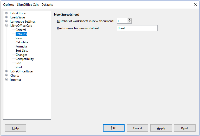
When you open a new spreadsheet it has, by default, one sheet named Sheet1. You can specify a different number of sheets to be created in a new document, or a different prefix name for new sheets, by going to Tools > Options > LibreOffice Calc > Defaults on the Menu bar (Figure 1).
Figure 1: Options > LibreOffice Calc > Defaults dialog
Sheets in Calc are managed using tabs located at the bottom of the spreadsheet.
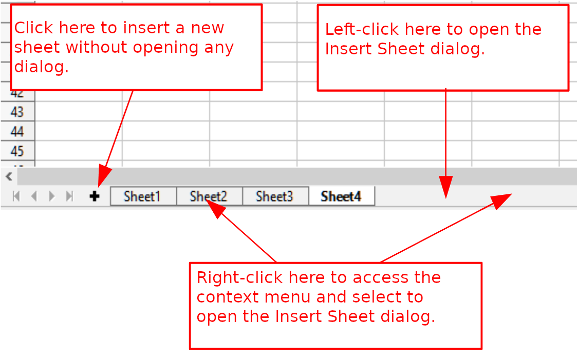
There are several ways to insert a new sheet. The fastest method is to click on the Add Sheet (+) icon located to the left of the sheet tabs, at the bottom of the spreadsheet. This inserts one new sheet without opening any dialog, with a default name (Sheet2, for example) and with the new sheet’s tab positioned at the right hand end of the sheet tabs.
Use one of these other methods to insert more than one sheet, to rename the sheet at the same time, or to insert the sheet somewhere else in the sequence.
Left-click a sheet tab and select Sheet > Insert Sheet on the Menu bar. Calc displays the Insert Sheet dialog with the Before current sheet and New sheet options preselected.
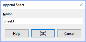
Select Sheet > Insert Sheet at End on the Menu bar. Calc displays the Append Sheet dialog.
Select Sheet > Insert Sheet from File on the Menu bar. Calc displays the Insert Sheet dialog with the Before current sheet and From file options preselected. It also displays a file browser dialog on top of the Insert Sheet dialog to enable you to first select the source file containing the sheet to be inserted.
Right-click on a sheet tab and select Insert Sheet in the context menu (Figure 2). Calc displays the Insert Sheet dialog with the Before current sheet and New sheet options preselected.
Left-click in the empty space at the right end of the line of sheet tabs (Figure 2). Calc displays the Insert Sheet dialog with the Before current sheet and New sheet options preselected.
Right-click in the empty space at the right end of the line of sheet tabs and select Insert Sheet in the context menu (Figure 2). Calc displays the Insert Sheet dialog with the Before current sheet and New sheet options preselected.
Figure 2: Creating a new sheet through the sheet tabs area
The above methods use either the Insert Sheet dialog (Figure 3) or the Append Sheet dialog (Figure 4).
On the Insert Sheet dialog, you can:
Choose whether to put the new sheet before or after the currently selected sheet tab.
Choose how many sheets to insert.
Choose the name for a single sheet (the Name field is unavailable if more than one sheet is to be inserted).
The From file option is described in “Inserting sheets from a different spreadsheet” (page 1).
Figure 3: Insert Sheet dialog
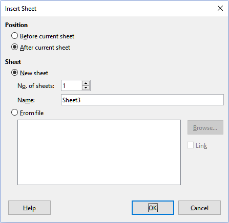
Figure 4: Append Sheet dialog
For John’s spreadsheet we need six sheets, one for each of his five accounts and one as a summary sheet. We also want to name each of these sheets for the account they represent: Summary, Checking Account, Savings Account, Credit Card 1, Credit Card 2, and Car Loan.
After creating a new spreadsheet with one sheet, we could:
Insert five new sheets and rename all six sheets afterwards
Rename the existing sheet, then insert the five new sheets one at a time, renaming each new sheet during the insert step.
To insert sheets and rename them afterwards:
1) Make sure that the correct sheet tab is selected and open the Insert Sheet dialog.
2) Choose the position for the new sheets (in this example, we use After current sheet).
3) Choose New sheet and enter 5 after No. of sheets:. Because you are inserting more than one sheet, the Name box is not available.
4) Click OK to insert the sheets.
For the subsequent steps to rename the sheets, see “Renaming sheets” (page 1).
To insert sheets and name them at the same time:
1) Rename the existing sheet as Summary, as described in “Renaming sheets” (page 1).
2) Make sure that the correct sheet tab is selected and open the Insert Sheet dialog.
3) Choose the sheet tab position for the new sheet (Before current sheet or After current sheet, as applicable).
4) Choose New sheet and enter 1 in the No. of sheets field. The Name box is now available.
5) In the Name box, type a name for this new sheet, for example Checking Account.
6) Click OK to insert the sheet.
7) Repeat steps to for each new sheet, giving them the names Savings Account, Credit Card 1, Credit Card 2, and Car Loan.
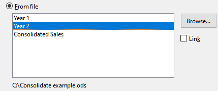
On the Insert Sheet dialog, you can also add a sheet from a different spreadsheet (for example, another Calc or Microsoft Excel file), by choosing the From file option. Click Browse, select the file using the file browser dialog, and click Open. A list of the available sheets in that file appears in the adjacent list box (Figure 5). Select the sheet to import (you can only import one at a time). If, after you select the file, no sheets appear, you probably selected an invalid file type (not a spreadsheet, for example).
Figure 5: From file area of Insert Sheet dialog showing file path and names of available sheets
If you prefer, select the Link option to insert the external sheet as a link instead of as a copy. This is one of several ways to include “live” data from another spreadsheet – see also “Linking to external data” below. The links can be updated manually to show the current contents of the external file using Edit > Links to External Files on the Menu bar. Alternatively the links can be updated automatically whenever the file is opened, depending on the options set on the dialog accessed by selecting Tools > Options > LibreOffice Calc > General on the Menu bar. The three options available in the Update links when opening section are Always (from trusted locations), On request, and Never.
To define trusted file locations, select Tools > Options > LibreOffice > Security > Macro Security (Trusted Sources tab) on the Menu bar. This is useful if you want to use macros in your spreadsheet. For more information about macros see Chapter 12, Macros.
Sheets can be renamed at any time. To give a sheet a more meaningful name:
Enter the name in the Name box when you create the sheet.
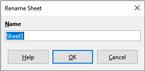
Double-click on the relevant sheet tab and replace the existing name through the Rename Sheet dialog.
Right-click on the relevant sheet tab, select Rename Sheet in the context menu, and replace the existing name through the Rename Sheet dialog.
Left-click on the relevant sheet tab, select Sheet > Rename Sheet on the Menu bar, and replace the existing name through the Rename Sheet dialog.
Figure 6: Rename Sheet dialog
A sheet name cannot be empty and must not be a duplicate of an existing name.
Note
The following characters are not allowed in sheet names: colon (:), back slash (\), forward slash (/), question mark (?), asterisk (*), left square bracket ([), right square bracket (]). The apostrophe (') character is not allowed as the first or last character of the name.
Tip
In some LibreOffice Calc installations you can hold down the Alt key, click on the sheet name, and enter the new name directly.
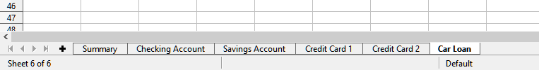
Your sheet tab area should now look like this.
Figure 7: Six renamed sheets
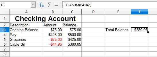
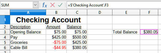
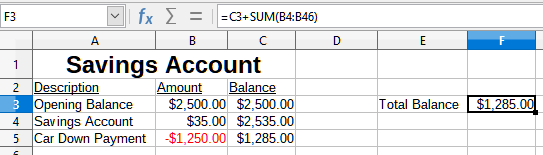
Now we will set up the account ledgers. This is just a simple summary that includes the previous balance plus the amount of the current transaction. For withdrawals, we enter the current transaction as a negative number so the balance gets smaller. A basic ledger is shown in Figure 8.
This ledger is set up in the sheet named Checking Account. The total balance is added up in cell F3. You can see the equation for it in the Formula bar. It is the summary of the opening balance, cell C3, and all of the subsequent transactions.
Figure 8: Checking ledger
On the Summary sheet we display the balance from each of the other sheets. If you copy the example in Figure 8 onto each of the five account sheets, the current balances will be in cell F3 of each sheet.
There are two ways to reference cells in other sheets: by entering the formula directly using the keyboard or by using the mouse.
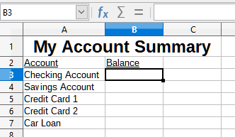
On the Summary sheet, set up a place for all five account balances, so we know where to put the cell reference. Figure 9 shows the Summary sheet with a blank Balance column. We want to place the reference for the Checking Account balance in cell B3.
Figure 9: Blank Summary sheet
To make the cell reference in cell B3, select the cell and follow these steps:
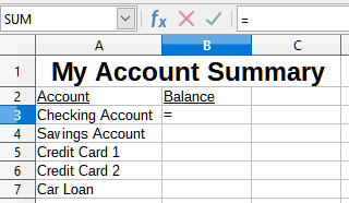
1) Click on the = icon next to the Input line on the Formula bar. The icons on the Formula bar change and an equals character appears in the Input line (Figure 10).
Figure 10: Equals character in Input line of Formula bar
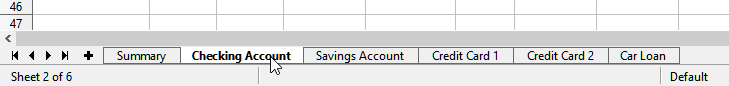
2) Now, click on the sheet tab for the sheet containing the cell to be referenced. In this case, that is the Checking Account sheet (Figure 11).
Figure 11: Click on the Checking Account sheet tab
3) Click on cell F3 (where the balance is) in the Checking Account sheet. The phrase $'Checking Account'.F3 should appear in the Input line (Figure 12) and the selected cell is surrounded by a colored border.
Figure 12: Cell reference selected
4) Click the Accept icon in the Input line of the Formula bar, or press the Enter key to finish.
5) The Summary sheet should now look like Figure 13.
Figure 13: Finished Checking Account reference
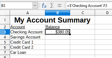
From Figure 13, you can deduce how the cell reference is constructed. The reference has two parts: the sheet name prefixed by a dollar symbol ($'Checking Account'), and the cell reference (F3). Notice that they are separated by a period. The default behavior of Calc is to insert the dollar symbol to form an absolute sheet reference while giving a relative cell reference.
Note
The sheet name is in single quotation marks because it contains a space, and the mandatory period (.) always falls outside any quotation marks.
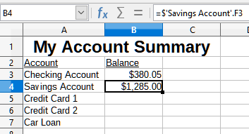
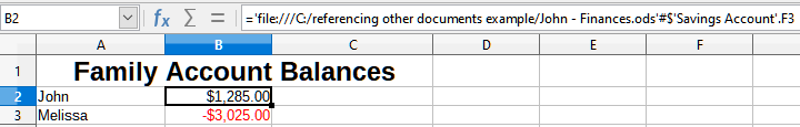
So, you can fill in the Savings Account cell reference by just typing it in. Assuming that the balance is in the same cell (F3) in the Savings Account sheet, the cell reference should be =$'Savings Account'.F3 (Figure 14).
Figure 14: Savings Account cell reference
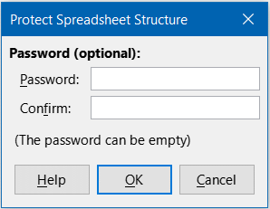
When you are satisfied with the structure of your spreadsheet in terms of its constituent sheets, select Tools > Protect Spreadsheet Structure on the Menu bar to lock that structure. Calc displays the Protect Spreadsheet Structure dialog (Figure 15). Press OK to inhibit the addition, deletion, repositioning, and renaming of sheets. To subsequently unlock the structure, select Tools > Protect Spreadsheet Structure again.
Figure 15: Protect Spreadsheet Structure dialog
John decides to keep his family account information in a different spreadsheet file from his own summary. Fortunately Calc can link different files together. The process is the same as described for different sheets in a single spreadsheet, but we add one more step to indicate which file the sheet is in.
To create the reference with the mouse, both spreadsheets need to be open.
1) If necessary, switch to the spreadsheet containing the cell in which the formula is going to be entered.
2) Select the cell in which the formula is going to be entered.
3) Click the = icon next to the Input line in the Formula bar.
4) Switch to the other spreadsheet (the process to do this may vary depending on which operating system you are using).
5) Select the sheet (Savings Account) and then the reference cell (F3); see Figure 16. You can press the keyboard Enter key at this point, or continue with steps and .
Figure 16: Selecting the Savings Account reference cell
6) Switch back to the original spreadsheet.
7) Click the Accept icon in the Formula bar.
Your spreadsheet should now resemble Figure 17.
You will get a good feel for the format of the reference if you look closely at the Input line in the Formula bar. Based on the contents of this line, you can create the reference using the keyboard.
Figure 17: Linked files
Typing the reference is simple once you know the format the reference takes. The reference has three parts to it:
Path and file name
Sheet name
Cell reference
In Figure 17, you can see that the general format for the reference is:
='file:///Path & File Name'#$'SheetName'.CellReference
Note
The reference for a file has three forward slashes ///, while the reference for a hyperlink has two forward slashes //. See “Using hyperlinks and URLs” below.
Hyperlinks can be used in Calc to jump to a different location from within a spreadsheet and can lead to other parts of the current file, to different files, or even to web pages.
Hyperlinks stored within a file can be either relative or absolute.
A relative hyperlink says, Here is how to get there starting from where you are now (meaning from the folder in which your current document is saved), while an absolute hyperlink says, Here is how to get there no matter where you start from.
An absolute link will stop working if the target is moved. A relative link will stop working if the start and target locations change relative to each other. For instance, if you have two spreadsheets in the same folder linked to each other and you move the entire folder to a new location, an absolute hyperlink will break but a relative one will not.
To change the way that Calc stores the hyperlinks in your file, select Tools > Options > Load/Save > General and in the Save area of the dialog, choose if you want URLs (Universal Resource Locators) saved relatively when referencing the file system, or the Internet, or both.
An absolute path such as c:\homepage\graphics\picture.gif would no longer function on a web server. Operating systems such as Unix or macOS do not recognize drive letters, and even if the folder homepage\graphics existed, your picture would not be available. It is better to use relative linking for file links. Relative linking is only possible when the document you are working on is on the same drive as the link destination.
Calc will always display an absolute hyperlink. Do not be alarmed when it does this even when you have saved a relative hyperlink. This ‘absolute’ target address will be updated if you move the file.
Note
HTML (Hypertext Markup Language) files containing links as relative to the file system that are to be uploaded to a web server require the files be in a file structure matching that of the web server. Otherwise, the links will point to the wrong folder.
Tip
When you rest the mouse pointer on a hyperlink, a help tip displays the absolute reference, because Calc uses absolute path names internally. The complete path and address can only be seen when you view the result of the HTML export (saving a spreadsheet as an HTML file), by loading the HTML file as text, or by opening it with a text editor.
You can insert a hyperlink into a Calc spreadsheet using one of these methods:
Place the text cursor at the point where you want to insert the hyperlink, or select the text that you want to put the hyperlink on. Select Insert > Hyperlink on the Menu bar, or click the Insert Hyperlink icon on the Standard toolbar, or press Ctrl+K, to access the Hyperlink dialog; see “Hyperlink dialog” below.
Drag-and-drop an item from the Navigator to the point where you want to insert the hyperlink (for example, a sheet or cell name).
Type the target web address or URL at the point where you want to insert the hyperlink. When you type text that can be used as a hyperlink (such as a website address or URL), Calc formats it automatically, creating the hyperlink and applying color to the text. If this does not happen, you can enable this feature using Tools > AutoCorrect Options > Options on the Menu bar and selecting URL Recognition. Make sure you start the hyperlink with http://, www., or ftp.; if you type only libreoffice.org for example, Calc will not recognize it as a hyperlink.
When you use the Hyperlink dialog to insert a hyperlink, you can select either a text hyperlink (Figure 18) or a button hyperlink (Figure 19). In both cases, the visible text can be different from the linked URL.
Figure 18: Example text hyperlink
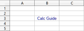
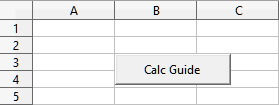
Figure 19: Example button hyperlink
To change the color of text hyperlinks, go to Tools > Options > LibreOffice > Application Colors on the Menu bar, scroll to Unvisited links and/or Visited links, pick the new colors, and click OK.
Note
This will change the color for all hyperlinks in all components of LibreOffice, which may not be what you want.
A button hyperlink is a type of form control. As with all form controls, it can be anchored or positioned by right-clicking on the button in design mode. More information about forms can be found in Chapter 18, Forms, of the Writer Guide.
To open a text hyperlink, do one of the following:
Ctrl-click with the cursor positioned over the hyperlink. This method only works if the Tools > Options > LibreOffice > Security > Security Options and Warnings > Options > Ctrl-click required to open hyperlinks option is selected.
Left-click with the cursor positioned over the hyperlink. This method only works if the Tools > Options > LibreOffice > Security > Security Options and Warnings > Options > Ctrl-click required to open hyperlinks option is not selected.
Right-click with the cursor positioned over the hyperlink and select the Open Hyperlink option in the context menu.
To open a button hyperlink, left-click the button. This method only works when the form design mode is deactivated; the status of this mode is controlled by clicking the Design Mode button on either the Form Controls toolbar or the Form Design toolbar.
You can insert and modify hyperlinks using the Hyperlink dialog (Figure 20). To display this dialog, choose Insert > Hyperlink on the Menu bar, or click the Insert Hyperlink icon on the Standard toolbar, or press Ctrl+K.
On the left side of the dialog, select one of the four categories of hyperlink:
Internet. The hyperlink points to a WWW (World Wide Web) or FTP (File Transfer Protocol) address.
Mail. The hyperlink points to an email address.
Document. The hyperlink points to a location in either the current document or another existing document.
New Document. Opening the hyperlink creates a new document.
Figure 20: Hyperlink dialog showing details for the Internet category
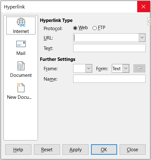
Figure 20 shows the Hyperlink dialog with the Internet category and the Web hyperlink type selected.
The Further Settings area is provided for all four hyperlink categories. The controls above the Further Settings area vary dependent on which of the four hyperlink categories is selected on the left side of the dialog.
A full description of all the choices and their interactions is beyond the scope of this chapter. The following is a summary of the most common choices used in Calc spreadsheets.
Internet
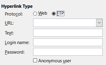
Web / FTP. Select the type of hyperlink. On selection of the FTP option, the controls above the Further Settings area change to those shown in Figure 21.
URL. Enter the required web address.
Text. Text specifies the text that will be visible to the user. If you do not enter anything here, Calc will use the full URL or path as the link text. Note that if the link is relative and you move the file, this text will not change, though the target will.
Login name. If necessary, enter your login to access the URL. Only applicable for FTP hyperlinks.
Password. If necessary, enter your password to access the URL. Only applicable for FTP hyperlinks.
Anonymous user. Mark this option to access the URL anonymously. Only applicable for FTP hyperlinks.
Figure 21: FTP specific controls on the Hyperlink dialog
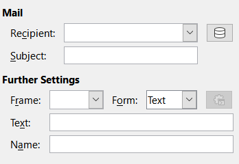
Recipient. Enter the email address of the recipient, or select the address from an existing database accessed by clicking the Data Sources button.
Subject. Enter the text to be used as the subject line of the message.
Figure 22: Mail controls on the Hyperlink dialog
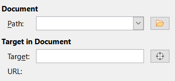
Document
Path. Specify the path of the file to be opened. Leave this blank if you want to link to a target in the same spreadsheet. The Open File icon opens a file browser for you to locate the document to be opened.
Target. Optionally specify the target in the document (for example a specific sheet). Click on the Target in Document icon to open a Navigator window where you can select the target, or if you know the name of the target, you can type it into the box.
Figure 23: Document controls on the Hyperlink dialog
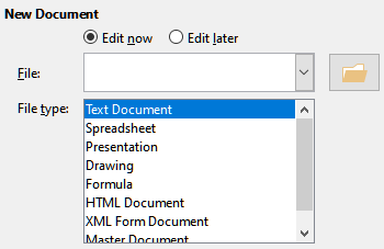
New Document
Edit now / Edit later. Specify whether to edit the newly created document immediately or just create it.
File. Enter the name of the file to be created. The Select Path icon opens a directory picker dialog.
File type. Select the type of document to be created (for example, text document, spreadsheet, or drawing).
Figure 24: New Document controls on the Hyperlink dialog
The Further Settings section on the Hyperlink dialog is common to all the hyperlink categories, although some choices are more relevant to some types of links and the Text option is omitted from this area for Internet hyperlinks.
Set the value of Frame to determine how the hyperlink will open. This applies to documents that open in a web browser. Options are _top, _parent, _blank, and _self.
Form specifies if the link is to be presented as text or as a button.
Text specifies the text that will be visible to the user. If you do not enter anything here, Calc will use the full URL or path as the link text. Note that if the link is relative and you move the file, this text will not change, though the target will.
Name is applicable to HTML documents. It specifies text that will be added as a NAME attribute in the HTML code behind the hyperlink.
Events button: opens the Assign Macro dialog. Select a macro to run when the link is clicked. This function is not covered further in this chapter.
To edit an existing text hyperlink, do any of the following:
If the Tools > Options > LibreOffice > Security > Security Options and Warnings > Options > Ctrl-click required to open hyperlinks option is selected, then click the cell containing the hyperlink. Select Insert > Hyperlink on the Menu bar, or click the Insert Hyperlink icon on the Standard toolbar, or press Ctrl+K.
Select the cell containing the hyperlink. In some cases you may need to select a nearby cell that does not contain a hyperlink and use the arrow keys to move the selection to the hyperlink cell. Select Insert > Hyperlink on the Menu bar, or click the Insert Hyperlink icon on the Standard toolbar, or press Ctrl+K.
Right-click on the hyperlink and select the Edit Hyperlink option in the context menu.
In all cases, Calc opens the Hyperlink dialog, where you can modify the characteristics of the hyperlink.
For a button hyperlink, the spreadsheet must have the form design mode enabled in order to edit the hyperlink. With the button selected, select Insert > Hyperlink on the Menu bar, or click the Insert Hyperlink icon on the Standard toolbar, or press Ctrl+K. Make your changes and click OK.
If you need to edit several hyperlinks, you can leave the Hyperlink dialog open until you have edited all of them. Be sure to click Apply after each one. When you are finished, click Close.
You can also edit a button hyperlink by selecting the button (with form design mode enabled), right-clicking, and selecting Control Properties in the context menu. Calc displays the Properties dialog. Modify the button text by editing the Label field and modify the link address by editing the URL field. Note that the Properties dialog do not contain an OK button, so after executing the desired changes, just close the dialog.
To remove a text or button hyperlink from the document completely, select it and use one of the many available deletion mechanisms (for example, select Edit > Cut on the Menu bar or Cut on the Standard toolbar; or right-click on the hyperlink and select Cut in the context menu; or press Backspace or Delete on the keyboard).
You can insert data from another document into a Calc spreadsheet as a link.
Two methods are described in this section: using the External Data dialog and using the Navigator. If your file has named ranges, database ranges, or named tables, and you know the name of the range or table you want to link to, using the External Data dialog is quick and easy. However, if the file has several ranges and tables, and you want to pick only one of them, you may not be able to easily determine which is which; in that case, the Navigator method may be easier.
Calc provides other methods for including linked data from external sources, see for example “Linking to registered data sources” below and “Dynamic Data Exchange (DDE)” below.
Note
When you open a file that contains links to external data, depending on your settings you may be prompted to update the links or they may be updated automatically. Depending on where the linked files are stored, the update process can take several minutes to complete.
The External Data dialog inserts data from an HTML, Calc, CSV (Comma-Separated Values), or Microsoft Excel file into the current sheet as a link. Calc utilizes a Web Page Query import filter, enabling you to insert tables from HTML documents.
To insert a link to external data using the External Data dialog:
1) Open the Calc document where the external data is to be inserted. This is the target document.
2) Select the cell where the upper left cell of the external data is to be inserted.
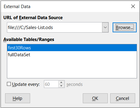
3) Choose Sheet > Link to External Data on the Menu bar. Calc displays the External Data dialog (Figure 25).
4) Type the URL of a web resource that is to be used as a data source, or type the address of a source file, or select an entry in the drop-down list, or select a source file from the file selection dialog accessed through the Browse button. For entries typed in, press Enter on completion.
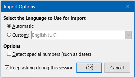
5) If you selected a HTML file as the data source at step , Calc displays the Import Options dialog (Figure 27). On this dialog you can choose the import language of the site. Select Automatic to let Calc import the data directly, or select Custom and choose from the drop-down list of languages available. You can also select the option to have Calc recognize special numbers, such as dates, on import.
Figure 25: External Data dialog
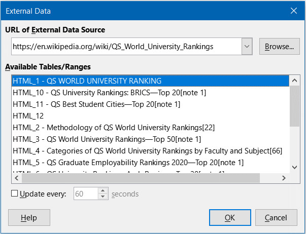
a) Click OK on the Import Options dialog. Calc loads the list of available tables/ranges into the Available Tables/Ranges area of the External Data dialog. The Web Page Query import filter can create names for cell ranges as they are imported. As much formatting as possible is retained while the filter intentionally does not import any images. The filter additionally creates two additional entries in the list: HTML_all to permit selection of the entire document and HTML_tables to permit selection of all the tables. Where a HTML table has a caption element, the text of the caption is appended to the associated entry in the list of available tables and ranges (Figure 26) and this helps identify a table of interest when there are many listed.
Figure 26: External Data dialog, with table captions
b) In the Available Tables/Ranges area, select the named ranges or tables you want to insert (hold Ctrl to select multiple entries). The OK button then becomes available.
Figure 27: Import Options dialog
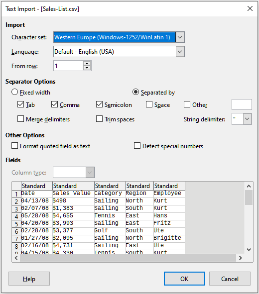
6) If you selected a CSV file as the data source at step , Calc displays the Text Import dialog (Figure 28). This dialog is described in detail in Chapter 1, Introduction. Click OK on the Text Import dialog and select CSV_all in the Available Tables/Ranges area of the External Data dialog. The OK button then becomes available.
7) If you selected a Calc or Microsoft Excel file as the data source at step , Calc populates the Available Tables/Ranges area of the External Data dialog with the list of range names and database ranges that are defined in the source file. Select the range names and database ranges that you want to insert (hold Ctrl to select multiple entries) and the OK button then becomes available.
Note
If the source Calc or Microsoft Excel spreadsheet contains no range names or database ranges, then you cannot use that document as the source file in the External Data dialog.
8) For all external data source file types, you can also specify that the data is refreshed at a specific frequency, defined in seconds.
9) Click OK to close the External Data dialog and insert the linked data.
Figure 28: Text import dialog
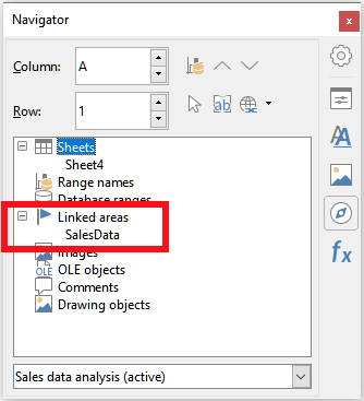
Calc adds the new entry to the Linked areas list in the Navigator (Figure 29). If you double-click this entry, Calc highlights the linked data within the sheet. When you hover the cursor over the entry, a tooltip indicates the file location of the linked data.
Figure 29: Linked areas in the Navigator
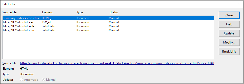
To view a list of all external data links in the spreadsheet, select Edit > Links to External Files on the Menu bar. Calc displays the Edit Links dialog (Figure 30).
Figure 30: Edit Links dialog
Note
The Edit Links dialog can display information about other links that were not created using the External Data dialog.
For links that have been created using the External Data dialog, you can access that dialog again by selecting the link on the Edit Links dialog and clicking the Modify button, or double-clicking the link. If you click Break Link and confirm that you want to remove the selected link, the previously-linked data becomes embedded in the spreadsheet. Click Update to refresh the linked data in the target file so that it matches that in the source file.
Note
The Status column on the Edit Links dialog always shows Manual for a link created using the External Data dialog. The status shown in this column does not reflect the setting of the Update every … seconds option on the External Data dialog.
You can also use the Navigator dialog or the Navigator deck of the Sidebar to link external data. Access the Navigator dialog by selecting View > Navigator on the Menu bar, or pressing F5. See Chapter 1, Introduction, for more details about the Navigator.
To insert a link to external data using the Navigator:
1) Open the Calc spreadsheet in which the external data is to be inserted (target document).
2) Open the document from which the external data is to be taken (source document) in Calc. The source document does not need to be a Calc file; it could, for example, be a Microsoft Excel file, an HTML file, or a CSV file. In the case of a HTML file, Calc displays the Import Options dialog (Figure 27) before opening the file.
3) In the target document, open the Navigator (Figure 31). This illustration shows the Navigator for a new file called Untitled 1, which currently has no range names, database ranges, or linked areas.
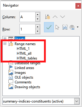
4) At the bottom of the Navigator, select the source document in the drop-down menu (Figure 32). In this case the source is called summary-indices-constituents and the file contains three range names which are highlighted with a red box. You may need to click the + icon at the left of the Range names field to view the names.
Figure 31: Navigator for target file
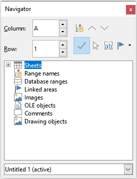
Figure 32: Navigator for source file
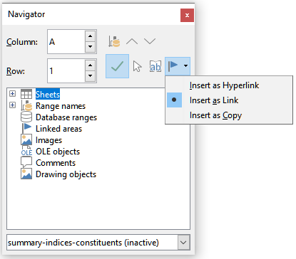
5) In the Navigator, select the Insert as Link option in the Drag Mode menu, as shown in Figure 33.
You can also change the drag mode by right-clicking on a range name and selecting the required option in the context menu.
Tip
The graphic on the Drag Mode icon on the Navigator changes to reflect the currently selected drag mode.
Figure 33: Select Insert as Link from Drag Mode menu
6) Select the required Range names or Database ranges entry and drag it from the Navigator into the target document, to the cell where you want the upper left cell of the data range to be.
7) Re-select the target document in the drop-down menu at the bottom of the Navigator. Instead of a + icon next to Range names, it shows a + icon next to Linked areas. Click the + icon to see the entry dragged across from the source document, similar to Figure 29.
Calc’s Web Page Query import filter gives names to the data ranges (tables) it finds in a web page, starting from HTML_1. It also creates two additional range names:
HTML_all – designates the entire document
HTML_tables – designates all HTML tables in the document
If any of the data tables in the source HTML document have been given meaningful names (using the ID attribute on the TABLE tag), those names appear in the Range names list, along with the ranges Calc has sequentially numbered.
If the data range or table you want is not meaningfully named, how can you tell which one to select?
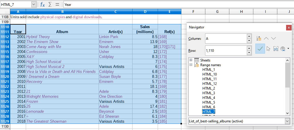
Go to the source document, which you opened in Calc. In the Navigator, double-click on a range name: that range is highlighted on the sheet. The example in Figure 34 shows a table of best-selling albums of recorded music by year worldwide and was extracted from Wikipedia’s List of best-selling albums page (https://en.wikipedia.org/wiki/List_of_best-selling_albums).
Figure 34: Using the Navigator to find a data range name
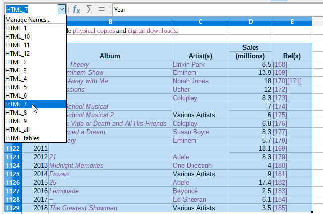
If the Formula bar is visible, the range name is also displayed in the Name Box at the left end (Figure 35). The range name can be selected in the drop-down list to highlight it on the page.
Figure 35: Using the Name Box to find a data range name
You can access a variety of databases and other data sources and link them into Calc documents.
First you need to register the data source with LibreOffice. To register means to tell LibreOffice what type of data source it is and where the file is located. The way to do this depends on whether or not the data source is a database in *.odb format.
To register a data source that is in *.odb format:
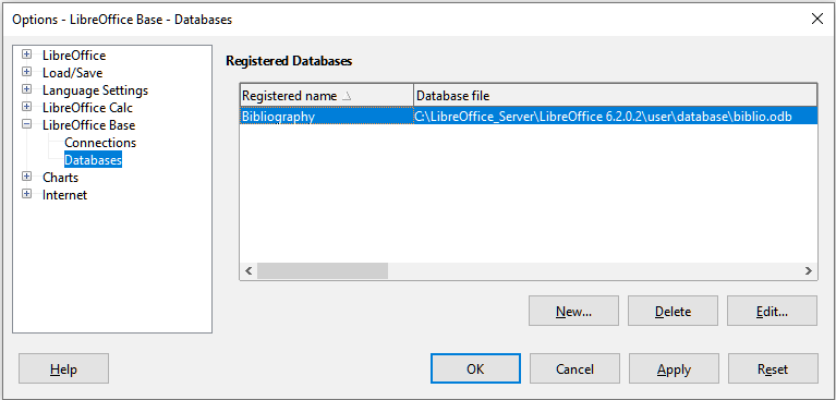
1) Select Tools > Options > LibreOffice Base > Databases on the Menu bar. Calc displays the dialog shown in Figure 36.
Figure 36: Options – LibreOffice Base – Databases dialog
2) Click the New button to open the Create Database Link dialog (Figure 37).
Figure 37: Create Database Link dialog
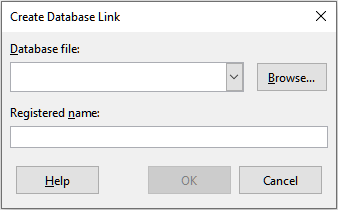
3) Enter the location of the database file, select a database file in the drop-down list, or click Browse to open a file browser and select the database file.
4) Type a name to use as the registered name for the database and click OK. The database is added to the list of registered databases and LibreOffice uses the registered name to access the database.
Note
The OK button on the Create Database Link dialog is enabled only when both the Database file and Registered name fields are filled in.
To register a data source that is not in *.odb format:
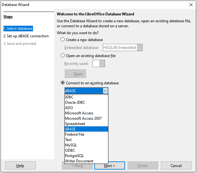
1) Choose File > New > Database on the Menu bar to open the Database Wizard (Figure 38). For more about the Database Wizard, see Chapter 2, Creating a Database, of the Base Handbook.
2) Select Connect to an existing database and select the appropriate database type in the drop-down menu. The choices for database type depend on your operating system. For example, Microsoft Access and other Microsoft products are not among the choices if you are using Linux. The example database type menu shown in Figure 38 relates to a Windows 10 installation.
Note
The exact interactions required to connect to a database vary depending on the type of database. Steps and assume that you selected dBASE at step .
3) Click Next. Type the path to the folder where the dBase files are stored or click Browse and use the folder selection dialog to navigate to the relevant folder before clicking the Select Folder button.
4) Click Next. Select Yes, register the database for me, but clear the Open the database for editing checkbox.
5) Click Finish. Name and save the database in the location of your choice.
Note
The above steps create a *.odb format database based on the content of the original dBASE database. The original dBASE database remains unchanged.
Figure 38: Database Wizard
Once a data source has been registered, it can be used by any LibreOffice component (for example, Calc or Writer).
Open a document in Calc. To view the data sources available, select View > Data Sources on the Menu bar, or press Ctrl+Shift+F4. Calc opens the Data Source window above the spreadsheet.
The Data Source window has four main components:
The Table Data toolbar
The Table Data toolbar (Figure 39) is by default located at the top of the Data Source window.
Figure 39: Table Data toolbar

The Table Data toolbar provides the following icons, from left to right:
Save current record
Edit Data
Cut
Copy
Paste
Undo
Find Record
Refresh
Sort
Sort Ascending
Sort Descending
AutoFilter
Apply Filter
Standard Filter
Reset Filter/Sort
Data to Text
Data to Fields
Mail Merge
Data Source of Current Document
Explorer On/Off
The Data Source Explorer
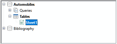
The Data Source Explorer (Figure 40) is by default located on the left side of the Data Source window, below the Table Data toolbar.
The Data Source Explorer provides a list of the registered databases, which by default includes the built-in Bibliography database.
To view each database, click on the expand icon to the left of the name of the database. This has already been done for the Automobiles database in Figure 40. Click on the expand icon left of Tables to view the individual tables within the selected database; similarly you can click on the expand icon left of Queries to view the individual queries within the selected database. Click on the name of a table to view all the records held in that table.
Figure 40: Data Source Explorer
Data records for selected table
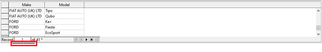
The data records for the selected table are displayed in the area at the right side of the Data Source window, below the Table Data toolbar.
Figure 41: Data Source window records
To see more columns in this area, you can click the Explorer On/Off icon on the Table Data toolbar to hide the Data Source Explorer. Click again to show it back.
Below the data records is a navigation bar, which shows which record is selected and the total number of records. This provides the following buttons, from left to right:
First record
Previous record
Next record
Last record
Add new record
A horizontal scroll bar appears when the available columns do not all fit in the visible area. A vertical scroll bar appears when the available data records do not all fit in the visible area.
Show / hide window
At the bottom center of the Data Source window is a control to hide and show the entire window. This control is highlighted with a red box in Figure 41.
Only registered Data Sources can be edited in the Data Source window.
In editable data sources, records can be edited, added, or deleted. If you cannot save your edits, you need to open the database in Base and edit it there; see “Launching Base to work on data sources” below. You can also hide columns and make other changes to the display.
You can launch LibreOffice Base at any time from the Data Source Explorer. Right-click on a database, Tables, a table name, Queries, or a query name, and then select Edit Database File in the context menu. Once in Base, you can edit, add, and delete tables, queries, forms, and reports.
For more about using Base, see Chapter 8, Getting Started with Base, in the Getting Started Guide, or the Base Guide.
Data from a table displayed on the right side of the Data Source window can be placed into a Calc document in a variety of ways.
You can select a single cell, a single row, or multiple rows in the Data Source window and drag and drop the data into the spreadsheet. The data is inserted at the place where you release the mouse button. If you selected one or more rows, Calc will also include the column headings above the data you insert. To select the rows of data you want to add to the spreadsheet:
1) Click the gray box to the left of the first row you want to select. That row is highlighted.
2) To select multiple adjacent rows, hold down the Shift key while clicking the gray box of the last row you need.
3) To select multiple separate rows, hold down the Control key while selecting each row. The selected rows are highlighted.
4) To select all the rows, click the gray box in the upper left corner. All rows are highlighted.
An alternative method uses the Data to Text icon on the Table Data toolbar and will include the column headings above the data you insert:
1) Click the cell of the spreadsheet which you want to be the top left of your data, including the column names.
2) Select the rows of data you want to add to the spreadsheet, as described in the previous paragraph.
3) Click the Data to Text icon in the Table Data toolbar to insert the data into the spreadsheet cells.
You can also drag the data source column headings (field names) onto your spreadsheet to create a form for viewing and editing individual records one at a time. Follow these steps:
1) Drag and drop the gray box at the top of the column (containing the field name you wish to use) to where you want the record to appear in the spreadsheet.
2) Repeat step until you have moved all of the fields you need to where you want them.
3) Close the Data Source window by selecting View > Data Sources on the Menu bar or pressing Ctrl+Shift+F4.
4) Save the spreadsheet and select Edit > Edit Mode on the Menu bar, or press Ctrl+Shift+M, to make the spreadsheet read-only.
5) Select File > Reload on the Menu bar. All of the fields will show the value for the data of the first record of the data source that you selected.
6) Select View > Toolbars > Form Navigation to show the Form Navigation toolbar (Figure 42). By default, this toolbar opens at the bottom of the Calc window, just above the Status bar.
Figure 42: Form Navigation toolbar

7) Click the arrows on the Form Navigation toolbar to view the different records of the table. The toolbar indicates which record is currently displayed and the total number of records available. The current record number changes as you move through the records and the data in the spreadsheet fields updates to correspond to the data for that particular record number.
From left to right, the Form Navigation toolbar provides the following interactions:
Find Record (provides access to the Record Search dialog)
Absolute Record (type in the number of the required record)
First Record
Previous Record
Next Record
Last Record
New Record
Save Record
Undo
Delete Record
Refresh
Refresh Control
Sort
Sort Ascending
Sort Descending
AutoFilter
Apply Filter
Form-Based Filters
Reset Filter/Sort
Data source as Table
Spreadsheets can be embedded in other LibreOffice files and vice versa. This is often used in Writer or Impress documents so that Calc data can be used in a text document or a presentation. You can embed the spreadsheet as either an OLE (Object Linking and Embedding) or DDE (Dynamic Data Exchange) object. The difference between a DDE object and a Linked OLE object is that a linked OLE object can be edited from the document in which it is added as a link, but a DDE object cannot.
For example, if a Calc spreadsheet is pasted into a Writer document as a DDE object, then the spreadsheet cannot be edited in the Writer document. But if the original Calc spreadsheet is updated, the changes are automatically made in the Writer document. If the spreadsheet is inserted as a Linked OLE object into the Writer document, then the spreadsheet can be edited in Writer as well as in the Calc document and both documents are in sync with each other.
The major benefit of an OLE object is that it is quick and easy to edit its contents just by double-clicking on it. You can also insert a link to the object that will appear as an icon rather than an area showing the contents itself.
OLE objects can be linked to a target document or embedded in the target document. Linking inserts information which will be updated with any subsequent changes to the original file, while embedding inserts a static copy of the data. If you want to edit the embedded spreadsheet, double-click on the object.
Note
If your OLE object is empty, inactive, and not displayed as an icon, then it will be transparent.
To embed a spreadsheet as an OLE object in a presentation:
1) Place the cursor in the document at the location where you want the OLE object to be.
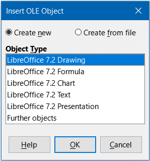
2) Select Insert > Object > OLE Object on the Menu bar. Impress opens the Insert OLE Object dialog shown in Figure 43, with the Create new option selected by default.
3) You can either create a new OLE object or create the OLE object from an existing file.
To create a new object:
1) Select the Create new option and select the required option from those available in the Object Type list. In this example, you would select LibreOffice 7.2 Spreadsheet.
2) Click OK.
3) LibreOffice places an empty container in the slide, ready for you to enter information. By default the Menu bar changes to reflect the Calc Menu bar; when you click on the slide, anywhere outside the spreadsheet area, the Menu bar reverts to the Impress Menu bar.
Figure 43: Insert OLE Object dialog with Create new option selected
After clicking outside the spreadsheet area, double-click on the OLE object to re-enter the edit mode of the object. The application devoted to handling that type of file (Calc in our example) will open the object.
To save the inserted spreadsheet:
1) Click anywhere outside the spreadsheet to leave the edit mode.
2) Right-click on the spreadsheet and select Save Copy as in the context menu or select Edit > Object > Save Copy as on the Menu bar.
3) Choose the name of the new file and the folder in which it will be saved.
4) Click the Save button.
Note
If the object inserted is handled by LibreOffice, then the transition to the program to manipulate the object will be seamless; in other cases the object opens in a new window and an option in the File menu becomes available to update the object you inserted.
To insert an existing object:
1) To create on OLE object from an existing file, select the Create from file option. The Insert OLE Object dialog changes to that shown in Figure 44.
Figure 44: Insert OLE Object dialog with Create from file option selected
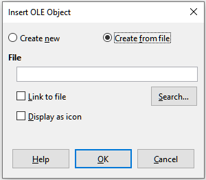
2) Click Search, select the required file in the file browser, and then click Open.
Note
This facility is not limited to LibreOffice files; you can create OLE objects using existing files from many other applications.
3) To insert the object as a link to the original file, select the Link to file option. Otherwise, the object will be embedded in your document.
4) If you want the object to appear as a selectable icon, rather than a section of your file, select the Display as icon option.
5) Click OK. A section of the inserted file is shown in the document. If your source spreadsheet has multiple sheets, it’s possible to navigate between them in the edit mode.
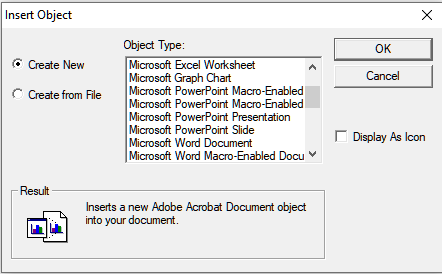
Under Windows, when you select the Create new option on the Insert OLE Object dialog, there is an extra entry Further objects in the Object Type list.
1) Double-click on the entry Further objects to open the Insert Object dialog (Figure 45).
2) Select Create New to insert a new object of the type selected in the Object Type list, or select Create from File to create a new object from an existing file.
Figure 45: Inserting an OLE object under Windows
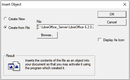
3) If you choose Create from File, the layout of the Insert Object dialog changes to that shown in Figure 46. Click Browse and choose the file to insert. The inserted file object is editable by the Windows program that created it.
4) Click OK.
Figure 46: Insert OLE object from a file under Windows
If the OLE object is not linked, it can be edited in the new document. For instance, if you insert a spreadsheet into a Writer document, you can essentially treat it as a Writer table (with a little more power). To edit it, double-click on it.
If the spreadsheet OLE object is linked and you change it in Writer, it will change in Calc; if you change it in Calc, it will change in Writer. This can be a very powerful tool if you create reports in Writer using Calc data, and want to make a quick change without opening Calc.
Note
You can only edit one copy of a spreadsheet at a time. If you have a linked OLE spreadsheet object in an open Writer document and then open the same spreadsheet in Calc, the Calc spreadsheet will be a read-only copy.
DDE is an acronym for Dynamic Data Exchange, a mechanism whereby selected data in document A can be pasted into document B as a linked, ‘live’ copy of the original. It would be used, for example, in a report written in Writer containing time‑varying data, such as sales results sourced from a Calc spreadsheet. The DDE link ensures that, as the source spreadsheet is updated so is the report, thus reducing the scope for error and reducing the work involved in keeping the Writer document up to date.
DDE is a predecessor of OLE. With DDE, objects are linked through file reference, but not embedded. You can create DDE links either within Calc cells in a Calc sheet, or in Calc cells in another LibreOffice doc such as in Writer.
Creating a DDE link in Calc is similar to creating a cell reference. The process is a little different, but the result is the same. Carry out the following steps to create a DDE link from one Calc spreadsheet to another:
1) In Calc, open the spreadsheet that contains the original data that you want to link to.
2) Select the cells that you want to make the DDE link to.
3) Copy the cells to the clipboard by selecting Edit > Copy on the Menu bar, or clicking the Copy icon on the Standard toolbar, or right-clicking the selected area and selecting Copy in the context menu, or pressing Ctrl+C.
4) Open the second spreadsheet that will contain the linked data.
5) Click in the top left cell of the area in the second spreadsheet where you want the linked data to appear.
6) On the second spreadsheet, select Edit > Paste Special > Paste Special on the Menu bar, or right-click the top left cell of the area and select Paste Special > Paste Special in the context menu, or press Ctrl+Shift+V.
7) Calc displays the Paste Special dialog (Figure 47).
8) Select the As Link option on the Paste Special dialog (highlighted with a red box on Figure 47) and then click OK.
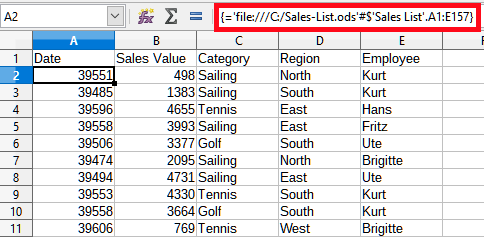
9) If you now click on one of the linked cells you will see that the Formula bar shows a reference beginning with the characters {=’. See Figure 48 for an example, highlighted with a red box.
10) Save and close both spreadsheets.
If you subsequently edit the original cells in their spreadsheet and save the changes, next time you open the spreadsheet containing the linked cells, the values in those linked cells will update to reflect the latest values of the original cells.
Figure 47: Paste Special dialog
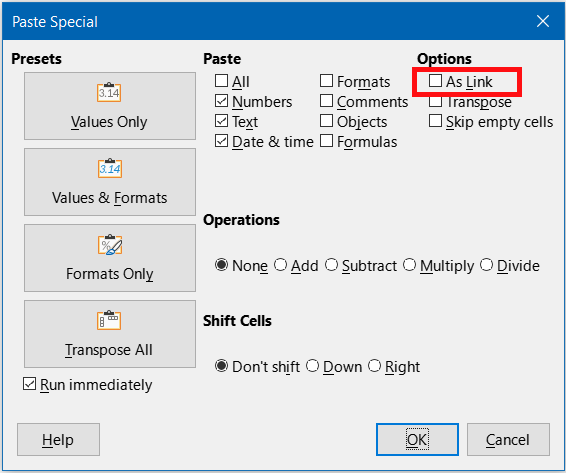
Figure 48: Example of DDE link to another Calc spreadsheet
Note
When you open a spreadsheet containing linked data, you may get a warning message indicating that automatic update of external links has been disabled. You will need to click the associated button to allow updating of the linked cells. You can avoid this message and interaction by making sure that the spreadsheet containing the original data is in a trusted file location and that the option is selected to always update links from trusted locations when opening. Check these settings via Tools > Options > LibreOffice > Security > Macro Security (Trusted Sources tab) and Tools > Options > LibreOffice Calc > General (Update links when opening section) respectively.
The process for creating a DDE link from Calc to Writer is similar to creating a link within Calc. You can check more details of this feature in Chapter 19, Spreadsheets, Charts, Other Objects of the Writer Guide.
1) In Calc, select the cells to make the DDE link to. Copy them.
2) Go to the place in your Writer document where you want the DDE link. Select Edit > Paste Special > Paste Special.
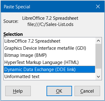
3) Writer displays its Paste Special dialog (Figure 49).
4) Select the Dynamic Data Exchange (DDE link) option in the Selection list.
5) Click OK.
6) Now the link has been created in Writer. When the Calc spreadsheet is updated, the table in Writer is automatically updated.
Figure 49: Paste Special dialog in Writer, with DDE link selected
The XML Source feature allows a user to import data from arbitrarily structured XML content into cells in an existing spreadsheet document. It allows XML content to be imported either partially or in full, depending on the structure of the XML content and the map definitions that the user defines. The user can specify multiple non-overlapping sub-structures to be mapped to different cell positions within the same document, and can select to import either element contents, attribute values, or both.
Note:
The XML Source feature currently allows you to import XML data as a one-time event; it will not store the information about the data source once the data is imported.
Suppose that you have sales data in an XML file, such as the following:
<sales>
<sale>
<date>01/19/08</date>
<value>$2,032</value>
<category>Golf</category>
<region>West</region>
<employee>Brigitte</employee>
</sale>
<sale>
<date>01/25/08</date>
<value>$3,116</value>
<category>Sailing</category>
<region>East</region>
<employee>Hans</employee>
</sale>
<sale>
<date>01/26/08</date>
<value>$2,811</value>
<category>Tennis</category>
<region>South</region>
<employee>Fritz</employee>
</sale>
</sales>
To import this data into your Calc spreadsheet, take the following steps:
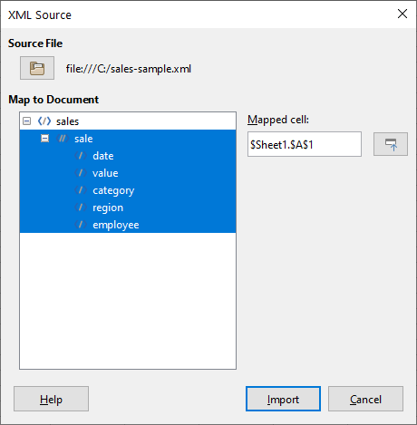
1) Select Data > XML Source. Calc displays the XML Source dialog (Figure 50).
2) Click the icon in the Source File area at the top of the dialog. Calc displays the Open dialog, which lets you specify the path to the XML file that you wish to import into your document.
3) Navigate to the correct folder, select the required file, and click the Open button.
4) Calc reads the content of the specified file and then populates the Map to Document area on the XML Source dialog to show the structure of the XML, as can be seen in Figure 51. The Map to Document area is described further below.
5) In the case of our example data, select sale in the Map to Document area. This will import all <sale> entries within the XML content into the spreadsheet.
6) Click on the cell at the top left of the area where the data is to appear in your spreadsheet. In the case of our example, click cell A1. A tellback of the cell clicked appears in the Mapped cell text box.
7) The contents of the XML Source dialog should now look like that shown in Figure 51.
8) Click the Import button. This action starts the import process based on the link definitions that the user has provided. Once the import finishes, the dialog will close.
Figure 50: XML Source dialog (on initial display)
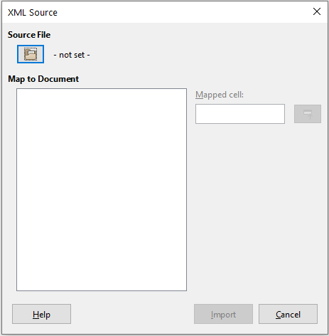
Figure 51: XML Source dialog (populated)
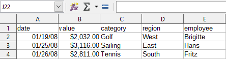
Calc will place the XML content into the specified position in the spreadsheet, as shown in Figure 52.
Figure 52: Imported XML content
The Map to Document area of the XML Source dialog shows the structure of the source XML content as a tree. It is initially empty and gets populated when you specify the source file.
Each element in the tree can be one of three types:
Attribute, represented by the symbol @.
Single non-recurring element, represented by the symbol </>. A non-recurring element is an element that can only occur once under the same parent. It is mapped to a single cell in the document.
Recurring element, represented by the symbol <//>. A recurring element is an element that can appear multiple times under the same parent. It serves as an enclosing parent of a single record entry of multiple record entries. These entries are imported into a range whose height equals the number of entries plus one additional header row.
The Mapped cell field specifies the position of a cell in the document that an element or an attribute is linked to. If it is a non-recurring element or an attribute, it simply points to the cell where the value of the linked element/attribute will get imported. If it is a recurring element, it points to the top-left cell of the range where the whole record entries plus header will get imported.