
Calc Guide 7.4
Chapter 1
Introduction
Using spreadsheets in LibreOffice
This document is Copyright ©2022 by the LibreOffice Documentation Team. Contributors are listed below. You may distribute it and/or modify it under the terms of either the GNU General Public License (https://www.gnu.org/licenses/gpl.html), version 3 or later, or the Creative Commons Attribution License (https://creativecommons.org/licenses/by/4.0/), version 4.0 or later.
All trademarks within this guide belong to their legitimate owners.
|
Skip Masonsmith |
Kees Kriek |
|
|
Barbara Duprey |
Gabriel Godoy |
Jean Hollis Weber |
|
John A Smith |
Christian Chenal |
Laurent Balland-Poirier |
|
Philippe Clément |
Pierre-Yves Samyn |
Shelagh Manton |
|
Peter Schofield |
Cathy Crumbley |
Kees Kriek |
|
Steve Fanning |
Leo Moons |
Gordon Bates |
|
Felipe Viggiano |
Zbyszek Zak |
|
Please direct any comments or suggestions about this document to the Documentation Team’s forum at https://community.documentfoundation.org/c/documentation/loguides/ (registration is required) or send an email to: loguides@community.documentfoundation.org.
Note
Everything you post to a forum, including your email address and any other personal information that is written in the message, is publicly archived and cannot be deleted. E-mails sent to the forum are moderated.
Published October 2022. Based on LibreOffice 7.4 Community.
Other versions of LibreOffice may differ in appearance and functionality.
Some keystrokes and menu items are different on macOS from those used in Windows and Linux. The table below gives some common substitutions for the instructions in this document. For a more detailed list, see the application Help and Appendix A (Keyboard Shortcuts) to this guide.
|
Windows or Linux |
macOS equivalent |
Effect |
|
Tools > Options menu selection |
LibreOffice > Preferences |
Access setup options |
|
Right-click |
Control+click and/or right-click depending on computer setup |
Open a context menu |
|
Ctrl (Control) |
⌘ (Command) |
Used with other keys |
|
F11 |
⌘+T |
Open the Styles deck in the Sidebar |
Calc is the spreadsheet component of LibreOffice. You can enter data (usually numerical) in a spreadsheet and then manipulate this data to produce certain results.
Alternatively, you can enter data and then use Calc in a ‘What if...’ manner by changing some of the data and observing the results without having to retype the entire spreadsheet or sheet.
Other features provided by Calc include:
Functions, which can be used to create formulas to perform complex calculations on data.
Database functions to arrange, store, and filter data.
Data statistics tools, to perform complex data analysis.
Dynamic charts, including a wide range of 2D and 3D charts.
Macros for recording and executing repetitive tasks; scripting languages supported include LibreOffice Basic, Python, BeanShell, and JavaScript.
Ability to open, edit, and save Microsoft Excel spreadsheets.
Import and export of spreadsheets in multiple formats, including HTML, CSV, PDF, and Data Interchange Format.
Note
If you want to use macros written in Microsoft Excel using the VBA macro code in LibreOffice, you must first edit the code in the LibreOffice Basic IDE editor. For more information, see Chapter 13, Macros, in this guide or Chapter 13, Getting Started with Macros, in the Getting Started Guide.
Calc works with documents called spreadsheets. Spreadsheets consist of a number of individual sheets, each sheet containing cells arranged in rows and columns. A particular cell is identified by its row number and column letter.
Cells hold the individual elements – text, numbers, formulas, and so on – that make up the data to display and manipulate.
Each spreadsheet can have up to 10,000 sheets and each sheet can have a maximum of 1,048,576 rows and 16,384 columns.
When Calc is started, the main window opens (Figure 1). The various parts of this display are explained below.
Note
By default, Calc’s commands are grouped in menus and toolbars, as described in this section. In addition, Calc provides other user interface variations, displaying contextual groups of commands and contents. For more information, see Chapter 16, User Interface Variants.
Note
If any part of the Calc window in Figure 1 is not shown, you can display it using the View menu. For example, View > Status Bar on the Menu bar will toggle (show or hide) the Status Bar. It is not always necessary to display all of the parts shown; you can show or hide any of them as desired.
Figure 1: Calc main window
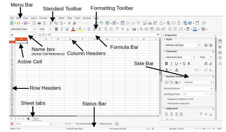
The Title bar, located at the top, shows the name of the current spreadsheet. When the spreadsheet is newly created, its name is Untitled X, where X is a number. When you save a spreadsheet for the first time, you are prompted to enter a name of your choice.
Under the Title bar is the Menu bar. When you choose one of the menus, a list of options appears. You can also modify the Menu bar, as explained in Chapter 15, Setting up and Customizing.
File – contains commands that apply to the entire document, such as Open, Save, Wizards, Export as PDF, Print, Digital Signatures, Templates.
Edit – contains commands for editing the document, such as Undo, Copy, Find and Replace, Track Changes.
View – contains commands for modifying how the Calc user interface looks, such as Toolbars, View Headers, Full Screen, Zoom.
Insert – contains commands for inserting elements into a spreadsheet, such as Image, Chart, Text Box, Headers and Footers.
Format – contains commands for modifying the layout of a spreadsheet, such as Cells, Page Style, AutoFormat Styles, Align Text.
Styles – contains options for applying and managing styles, such as Heading 1, Footnote, Manage Styles.
Sheet – contains commands for inserting and deleting elements and modifying the entire sheet, such as Delete Rows, Insert Sheet, Rename Sheet, Navigate.
Data – contains commands for manipulating data in your spreadsheet, such as Define Range, Sort, AutoFilter, Consolidate, Statistics.
Tools – contains functions to help check and customize a spreadsheet, for example Spelling, Share Spreadsheet, Macros, Options.
Window – contains two commands; New Window and Close Window. Also shows all open windows in other LibreOffice applications.
Help – contains links to LibreOffice Help (included with the software), User Guides, and other miscellaneous functions; for example Restart in Safe Mode, License Information, Check for Updates, About LibreOffice.
The scope of the Menu bar can be daunting for some people and even experienced users can forget where to look for rarely used functions. To quickly locate and run a command in the Menu bar, select Help > Search Commands or press Shift+Esc. Calc displays the dialog shown in Figure 2.
Figure 2: Search Commands dialog
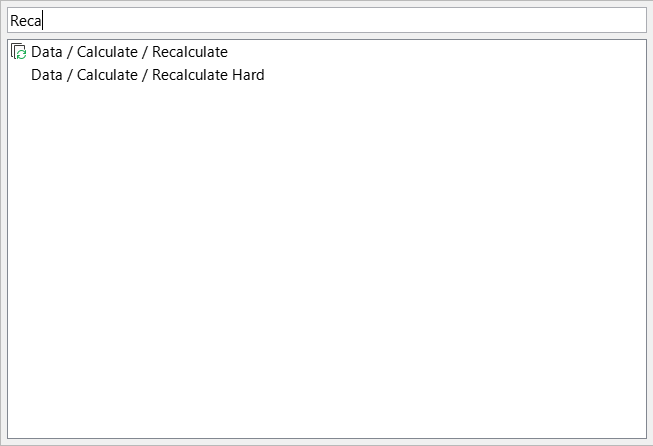
In the above example the pop-up is used to search for the available recalculate options, which appear in the lower area as soon as the letters “Reca” are typed in the upper area. The required option is run by clicking on it, or by using the arrow buttons on the keyboard to move through the options and then pressing the Enter key.
The default setting when Calc opens is for the Standard and Formatting toolbars to be docked at the top of the workspace (Figure 1).
Calc toolbars can be either docked (fixed in place), or floating, allowing you to move a toolbar to a more convenient location on your workspace. Docked toolbars can be undocked and moved to a different docked location or become floating toolbars. Likewise, floating toolbars can be docked.
The initial default is for all displayed toolbars to be locked in their docked positions. An individual toolbar can be unlocked, when a vertical handle is displayed at its left edge, and this handle can be used to drag the toolbar to a new screen position. To lock / unlock all toolbars at once, select View > Toolbars > Lock Toolbars (LibreOffice must be restarted to apply this change).
You can choose the single-toolbar alternative to the default double toolbar arrangement. It contains the most-used commands. To activate it, enable View > User Interface > Single Toolbar. Other variations are also available through View > User Interface.
For additional information on toolbars, see Chapter 1, Introducing LibreOffice, in the Getting Started Guide.
The default set of icons (sometimes called buttons) on toolbars provides a wide range of common commands and functions. You can also remove or add icons to toolbars. See Chapter 15, Setting up and Customizing, for more information.
Placing the mouse pointer over an icon, text box, or menu command, displays a small box called a tooltip that shows the name of the item’s function. To close a tooltip, move away from the underlying component or press the Esc key.
To see a more detailed explanation of an icon, text box, or menu command, do one of the following to open extended tips:
To activate extended tips just once: press Shift+F1.
To activate extended tips from the Menu bar: go to Help > What’s This? and hover the mouse pointer over an icon.
To turn extended tips on or off: go to Tools > Options > LibreOffice > General on the Menu bar and toggle the Extended tips checkbox.
The Formula Bar is located at the top of the Calc workspace. It is permanently docked in this position and cannot be used as a floating toolbar. However, it can be hidden or made visible by going to View > Formula Bar on the Menu bar.
Figure 3: Formula Bar

From left to right in Figure 3, the Formula Bar consists of the following:
Name Box – gives the current active cell reference using a combination of a letter and number, for example A1. The letter indicates the column and the number indicates the row of the selected cell. If you have selected a range of cells that is also a named range, the name of the range is shown in this box. You can also type a cell reference in the Name Box to jump to the referenced cell. If you type the name of a named range and press the Enter key, the named range is selected and displayed.
Function Wizard – opens a dialog from which you can search through lists of available functions and formulas. This can be very useful because it also shows how the functions are formatted.
Select Function – performs a calculation on the numbers in the cells above the selected cell and then places the result in it. If there are no numbers above the selected cell, then the calculation operates on the cells to the left. The calculation to be performed is selected from a drop-down menu containing options for Sum, Average, Min, Max, Count, CountA, Product, Stdev, StdevP, Var, and VarP. The Alt+= keyboard shortcut is equivalent to clicking the Select Function icon and selecting the Sum option.
Formula – inserts an equals (=) sign in the selected cell and the Input line, allowing a formula to be entered.
Input line – displays the contents of the selected cell (data, formula, or function) and allows you to edit the cell contents. To turn the Input line into a multi-line input area for very long formulas, click the Expand Formula Bar icon on the right or Click and drag between the Formula Bar and top of the Column Headers (when mouse pointer turns into a double arrow) to extend downwards. To edit inside the Input line area, click in the area, then type your changes. The height of the formula bar will be saved in your document.
You can also directly edit inside the cell by double-clicking on the cell. When you enter new data into a cell, the Select Function and Formula icons change to Cancel and Accept icons.
Note
In a spreadsheet, the term “function” covers much more than just mathematical functions. See Chapter 8, Using Formulas and Functions, for more information.
The Status Bar at the bottom of the workspace (Figure 4) provides information about the spreadsheet and convenient ways to quickly change some of its features. Most of the fields are similar to those in other components of LibreOffice. See Chapter 1, Introducing LibreOffice, in the Getting Started Guide for more information.
Figure 4: Status Bar
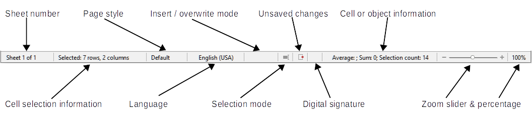
The fields on the Status Bar, from left to right, are as follows.
Sheet number
Cell selection information
Page style
Language
Insert / overwrite mode
Unsaved changes
Digital signature
Cell or object information
Zoom percentage
The Sidebar (Figure 5) is a mixture of toolbar and dialog. When opened (View > Sidebar or Ctrl+F5), it appears on the right side of the window. When entering or editing data in cells, the Sidebar consists of five decks: Properties, Styles, Gallery, Navigator, and Functions. Each deck has a corresponding icon on the Tab panel to the right of the Sidebar, allowing you to switch between them. These decks are described below. However, the Sidebar is context-sensitive and the number of decks and the content of each may change when you select objects such as images or charts.
Figure 5: Sidebar
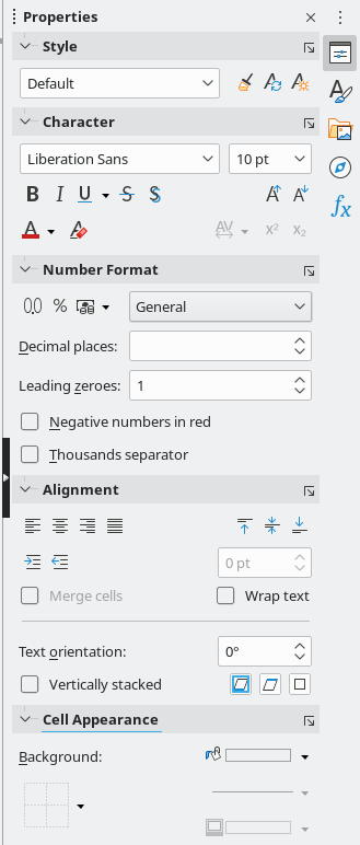
To the right side of the title bar of each open deck is a Close Sidebar Deck button, which closes the deck to leave only the Tab bar of the Sidebar open. Click any button in the Tab bar to toggle on / off the display of the associated deck.
To hide the Sidebar, or reveal it if already hidden, click on the left edge Hide/Show button. To adjust the deck width, drag on the left edge of the Sidebar.
The main section of the screen displays the cells in the form of a grid, with each cell located at the intersection of a column and a row.
At the top of the columns and the left end of the rows are a series of header boxes containing letters and numbers. The column headers use alphabetic characters that start with A and increase to the right. The row headers use numerical characters that start at 1 and increase down.
These column and row headers form the cell references that appear in the Name Box on the Formula Bar (Figure 3). If the headers are not visible on the spreadsheet, go to View > View Headers on the Menu bar.
When the mouse pointer lies over the grid of cells, the system default pointer is normally shown (typically an arrow pointer). However, a configuration option is available to switch to using the pointer shape defined in the icon theme (typically a fat cross). See Chapter 15, Setting up and Customizing for more information.
A spreadsheet file can contain many individual sheets. At the bottom of the grid of cells in a spreadsheet are sheet tabs (Figure 1). Each tab represents a sheet in a spreadsheet. You can create a new sheet by clicking on the plus sign to the left of the sheet tabs or by clicking in the blank space to the right of the sheet tabs.
Clicking on a tab makes an individual sheet active. When a sheet is active, the tab is highlighted. To select multiple sheets, hold down the Ctrl key while clicking on the sheet tabs.
To change the default name for a sheet (Sheet1, Sheet2, and so on):
1) Right-click on the sheet tab and select Rename Sheet in the context menu. In the dialog that opens, type in a new name for the sheet.
2) Click OK when finished to close the dialog.
To change the color of a sheet tab:
1) Right-click on the sheet tab and select Tab Color in the context menu to open the Tab Color dialog (Figure 6).
Figure 6: Tab Color dialog
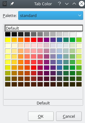
2) Select a color and click OK when finished to apply the color and close the dialog.
To add new colors to this color palette, see “Adding custom colors” in Chapter 15, Setting up and Customizing.
Creating and opening spreadsheets is identical to creating and opening documents in the other LibreOffice modules. For more information on creating and opening spreadsheets, see Chapter 1, Introducing LibreOffice, in the Getting Started Guide.
Calc documents can also be created from templates. For information on how to create and use templates, see Chapter 5, Using Styles and Templates, in this guide.
Comma-separated values (CSV) files are spreadsheet files in a text format where cell contents are separated by a character such as a comma or semi-colon. Each line in a CSV text file represents a row in a spreadsheet. Text is entered between quotation marks; numbers are entered without quotation marks.
1) Choose File > Open on the Menu bar, click the Open icon on the Standard toolbar, or press Ctrl+O and locate the CSV file that you want to open.
2) Select the file and click Open. By default, a CSV file has the extension .csv. However, some CSV files may have a .txt extension.
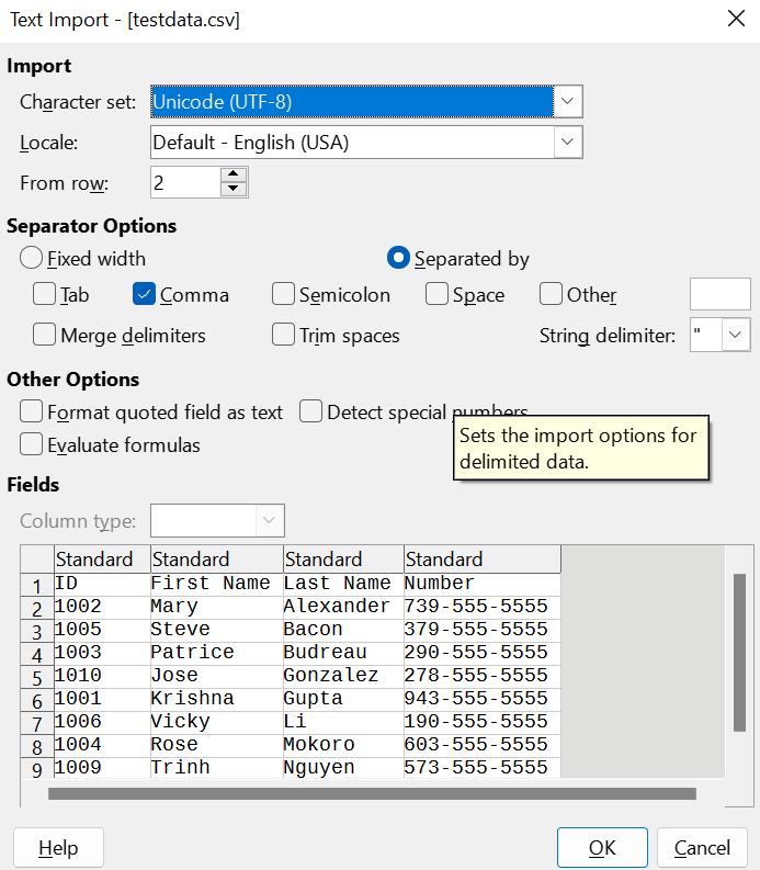
3) The Text Import dialog (Figure 7) opens. Here you can select options for importing a CSV file into a Calc spreadsheet.
4) Click OK to open and import the file.
The options for importing CSV files into a Calc spreadsheet are as follows:
Import
Character set – specifies the character set to be used in the imported file.
Language – determines how the number strings are imported. If Language is set to Default, Calc will use the language associated with the locale selected at Tools > Options > Language Settings > Languages > Formats. If another language is selected, that language will determine how numbers are treated.
From row – specifies which row the import starts with. The initial rows are visible in the preview window at the bottom of the dialog.
Separator Options
Fixed width – separates data into columns by a set number of characters. Click on the ruler that appears in the preview window to set the width.
Separated by – separates data into columns based on the separator defined here. Select Other to specify another character used to separate data into columns. This custom separator must also be contained in the data.
Merge delimiters – combines consecutive delimiters and removes blank data fields.
Trim spaces – removes starting and trailing spaces from within fields.
String delimiter – select a character to delimit text data.
Tip
CSV files can identify the separator to use by including a first row of sep=X or “sep=X” where X is the separator character. Set From row to 2 to import correctly.
Figure 7: Text Import dialog
Other options
Format quoted field as text – when this option is enabled, fields or cells whose values are entirely within quotes are imported as text.
Detect special numbers – when this option is enabled, Calc will automatically detect all number formats, including special number formats such as dates, time, and scientific notation. The selected language influences how such special numbers are detected, since different languages and regions many have different conventions for such special numbers.
When this option is disabled, Calc will detect and convert only decimal numbers. The rest, including numbers formatted in scientific notation, will be imported as text. A decimal number string can have digits 0–9, thousands separators, and a decimal separator. Thousands separators and decimal separators may vary with the selected language and region.
Evaluate formulas – when this option is enabled, fields that begin with an equals sign (=) will be imported and evaluated as a formula instead of as data.
Fields – shows how your data will look when it is separated into columns.
Standard – Calc determines the type of data.
Text – imported data are treated as text.
Date – imported data are treated as dates in the selected format – “DMY”, “MDY”, or “YMD”.
US English – numbers formatted in US English are searched for and included regardless of the system language. A number format is not applied. If there are no US English entries, the Standard format is applied.
Hide – the data in the column are not imported.
For information on how to save files manually or automatically, see Chapter 1, Introducing LibreOffice, in the Getting Started Guide. Calc can save spreadsheets in a range of formats and also export spreadsheets to PDF and XHTML file formats; see Chapter 7, Printing, Exporting, Emailing, and Signing, for more information.
If you need to send files to users who are unable to receive spreadsheet files in Open Document Format (ODF) (*.ods), which Calc uses as its default format, you can save a spreadsheet in another format.
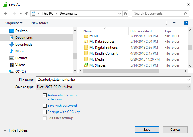
1) Select File > Save As on the Menu bar, click the down arrow at the right of the Save icon on the Standard toolbar and select Save As from the drop-down menu, or press Ctrl+Shift+S to open the Save As dialog (Figure 8).
2) In File name, if you wish, enter a new file name for the spreadsheet and select the folder where you want to save the file.
3) In the Save as type field, select from the drop-down menu the type of spreadsheet format you want to use. If Automatic file name extension is selected, the correct file extension for the spreadsheet format you have selected will be added to the file name.
4) Click Save.
Figure 8: The Save As dialog
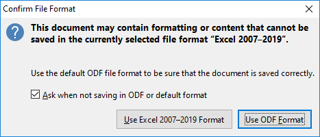
Each time a file is saved in a format other than ODF format, the Confirm File Format dialog opens (Figure 9). Click Use [xxx] Format to continue saving in the selected spreadsheet format or click Use ODF Format to save the spreadsheet in Calc’s default format. If you disable Warn when not saving in ODF or default format on Tools > Options > Load/Save > General on the Menu bar, the Confirm File Format dialog will no longer appear. You can also clear the checkbox Ask when not saving in ODF or default format on the dialog to stop the dialog appearing.
Figure 9: Confirm File Format dialog
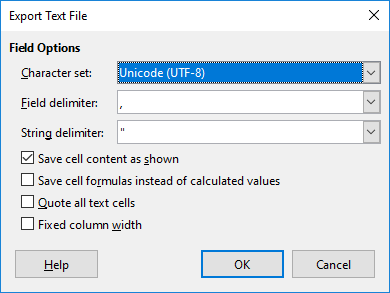
If you select Text CSV format (*.csv), the Export Text File dialog (Figure 10) opens. Here you can select the character set, field delimiter, string delimiter, and so on to be used for the CSV file.
Note
Once you have saved a spreadsheet in another format, all changes you make to the spreadsheet will now occur only in the format you are using because you have changed the name and file type of your document. If you want to go back to working with an *.ods version, you must save the file as an *.ods file.
Figure 10: Export Text File dialog
Tip
To have Calc save documents by default in a file format other than the default ODF format, go to Tools > Options > Load/Save > General. In the section named Default File Format and ODF Settings, next to Document type, select Spreadsheet, then next to Always save as, select your preferred file format, for example one of the available Microsoft Excel options.
To protect a spreadsheet and restrict who can open, read, and make changes to it, you have to use password protection. Password protection is common to all LibreOffice modules; for more information, see Chapter 1, Introducing LibreOffice, in the Getting Started Guide.
Calc provides many ways to navigate within a spreadsheet from cell to cell and sheet to sheet. You can generally use the method you prefer.
When a cell is selected or in focus, the cell borders are emphasized. When a group of cells is selected, the cell area is colored. The color of the cell border emphasis and the color of a group of selected cells depends on the operating system being used and uses your system’s highlight color.
Using the mouse – place the mouse pointer over the cell and click the left mouse button. To move the focus to another cell using the mouse, move the mouse pointer to the cell and click the left mouse button.
Using a cell reference – select or delete the existing cell reference in the Name Box on the Formula Bar (Figure 3 above). Type the reference of the cell you want to move to and press the Enter key. Cell references are case insensitive. Thus, typing a3 or A3 will move the focus to cell A3.
Using the Navigator – to open the Navigator (Figure 20), go to View > Navigator on the Menu bar, or press F5, or click the Navigator button on the Sidebar. Type the cell references into the Column and Row fields and press the Enter key.
Using the Enter key – pressing Enter moves the cell focus down one cell (by default). You can change the direction of this focus movement as described in the “Customizing the Enter key” section on page 1.
Pressing Shift+Enter moves the focus one cell in the opposite direction to that associated with the Enter key.
Using the Tab key – pressing Tab moves the cell focus one cell to the right. Pressing Shift+Tab moves the focus one cell to the left.
Using the arrow keys – pressing the arrow keys on the keyboard moves the cell focus in the direction of the arrow pressed.
Using Home, End, Page Up, and Page Down
Home moves the cell focus to the start of a row. Ctrl+Home moves the cell focus to the first cell in the sheet, A1.
The result of pressing End or Ctrl+End depends on the data contained in the sheet. To explain these key presses, it is helpful to define Rmax as the highest numbered row in the sheet that contains any data and Cmax as the rightmost column in the sheet that contains any data. Press End to move the cell focus along the current row to the cell in column Cmax. Press Ctrl+End to move the cell focus to the cell at the intersection of row Rmax and column Cmax. Note that in either case, the newly focused cell may not contain any data.
Page Down moves the cell focus down one complete screen display.
Page Up moves the cell focus up one complete screen display.
Each sheet in a spreadsheet is independent of the other sheets, though references can be linked from one sheet to another. There are four ways to navigate between different sheets in a spreadsheet.
Using the Navigator – when the Navigator is open (Figure 20), double-clicking on any of the listed sheets selects the sheet.
Using the keyboard – using key combinations Ctrl+Page Down moves one sheet to the right and Ctrl+Page Up moves one sheet to the left.
Using the mouse – clicking on one of the sheet tabs at the bottom of the spreadsheet selects that sheet.
Using the menu – go to Sheet > Navigate > To Previous Sheet / To Next Sheet to navigate to previous or next sheet. Sheet > Navigate > Go to Sheet brings up a dialog box that allows you to select a sheet or to search for a sheet by name.
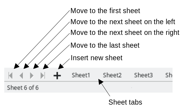
If there are many sheets in the spreadsheet, some of the sheet tabs may be hidden. If this is the case, use the four buttons to the left of the sheet tabs to move the tabs into view (Figure 11).
Note
The sheet tab arrows that appear on the left in Figure 11 are only active if there are more sheet tabs than can be displayed.
Figure 11: Navigating sheet tabs
Note
When you insert a new sheet into a spreadsheet, Calc automatically uses the next number in the numeric sequence as a name. Depending on which sheet is open when you insert a new sheet, your new sheet may not be in numerical order. It is recommended to rename sheets in a spreadsheet to make them more recognizable.
You can navigate a spreadsheet using the keyboard, by pressing a key or a combination of keys at the same time. For example, Ctrl+Home moves the focus to cell A1. Table 1 lists the keys and key combinations you can use for spreadsheet navigation in Calc.
Table 1. Keyboard cell navigation
|
Keyboard shortcut |
Cell navigation |
|
→/← |
Moves cell focus right/left one cell. |
|
↑/↓ |
Moves cell focus up/down one cell. |
|
Ctrl+→ / Ctrl+← |
If focus is on a blank cell, Ctrl+→ moves focus along the current row to the first cell on the right that contains data. If there is no cell on the right containing data, it moves focus along the current row to the last cell at the right of the sheet. If focus is on a blank cell, Ctrl+← moves focus along the current row to the first cell on the left that contains data. If there is no cell on the left containing data, it moves focus along the current row to the cell in column A of the sheet. If focus is on a cell containing data, Ctrl+→ normally moves focus along the current row to the cell at the right edge of the same data region. However, if there is a blank cell to the right of the original cell, focus is moved to the cell at the left edge of the next data region to the right. In this case, if there is no data region to the right, focus is moved along the current row to the last cell at the right of the sheet. If focus is on a cell containing data, Ctrl+← normally moves focus along the current row to the cell at the left edge of the same data region. However, if there is a blank cell to the left of the original cell, focus is moved to the cell at the right edge of the next data region to the left. In this case, if there is no data region to the left, focus is moved along the current row to the cell in column A of the sheet. |
|
Ctrl+↑ / Ctrl+↓ |
If focus is on a blank cell, Ctrl+↑ moves focus up the current column to the first cell that contains data. If there is no cell above containing data, it moves focus up the current column to the cell in row 1 of the sheet. If focus is on a blank cell, Ctrl+↓ moves focus down the current column to the first cell that contains data. If there is no cell below containing data, it moves focus down the current column to the last cell at the bottom of the sheet. If focus is on a cell containing data, Ctrl+↑ normally moves focus up the current column to the cell at the top edge of the same data region. However, if there is a blank cell above the original cell, focus is moved to the cell at the bottom edge of the next data region above. In this case, if there is no data region above, focus is moved up the current column to the cell in row 1 of the sheet. If focus is on a cell containing data, Ctrl+↓ normally moves focus down the current column to the cell at the bottom edge of the same data region. However, if there is a blank cell below the original cell, focus is moved to the cell at the top edge of the next data region below. In this case, if there is no data region below, focus is moved down the current column to the bottom of the sheet. |
|
Ctrl+Home / Ctrl+End |
A detailed description of these shortcuts is given on Page 1. |
|
Alt+Page Down / Alt+Page Up |
Moves focus one screen to the right/left (if possible). |
|
Ctrl+Page Down / Ctrl+Page Up |
Moves focus to the next sheet to the right/left in sheet tabs if there are more sheets in that direction. |
|
Tab / Shift+Tab |
Moves focus to the next cell on the right/left. |
|
Enter / Shift+Enter |
Moves focus down/up one cell (unless you have changed this action, as described in the following subsection). |
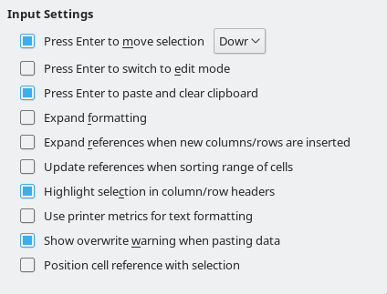
You can choose the direction in which the Enter key moves the cell focus by going to Tools > Options > LibreOffice Calc > General. Use the first three options under Input Settings (Figure 12) to change the Enter key settings. Select the direction cell focus moves from the drop-down list. Depending on the file being used or the type of data being entered, setting a different direction can be useful. The Enter key can also be used to switch into and out of editing mode. In Calc, when the content of a cell is copied to the clipboard, you can paste the information in another cell by pressing the Enter key; here you can disable this feature.
Figure 12: Customizing the Enter key
Click in the cell. You can verify the selection by looking in the Name Box on the Formula Bar (Figure 3).
A range of cells can be selected using the keyboard or the mouse.
To select a range of cells by dragging the mouse pointer:
1) Click in a cell.
2) Press and hold down the left mouse button.
3) Move the mouse to highlight the desired block of cells, then release the left mouse button.
To select a range of cells without dragging the mouse:
1) Click in the cell which is to be one corner of the range of cells.
2) Move the mouse to the opposite corner of the range of cells.
3) Hold down the Shift key and click.
To select a range of cells using Extending selection mode:
1) Click in the cell which is to be one corner of the range of cells.
2) Click in the Selection mode field on the Status Bar (Figure 4 above) and select Extending selection.
3) Click in the cell in the opposite corner of the range of cells.
Tip
Make sure to change back to Standard selection mode or you may find yourself extending a cell selection unintentionally.
To select a range of cells without using the mouse:
1) Select the cell that will be one of the corners in the range of cells.
2) While holding down the Shift key, use the cursor arrows to select the rest of the range.
To select a range of cells using the Name Box:
1) Click in the Name Box on the Formula Bar (Figure 3 above).
2) Enter the cell reference for the upper left-hand cell, followed by a colon (:), and then the lower right-hand cell reference, then press the Enter key. For example, to select the range that would go from A3 to C6, enter A3:C6.
To select a range of non-contiguous cells using the mouse:
1) Select the first cell or range of cells using one of the methods above.
2) Move the mouse pointer to the start of the next range or single cell.
3) Hold down the Ctrl key and click or click-and-drag to select another range of cells to add to the first range.
4) Repeat as necessary.
To select a range of cells using Adding selection mode:
1) Click in the Selection mode field on the Status Bar (Figure 4 above) and select Adding selection.
2) Click or click-and-drag to select ranges of cells to add to the selection.
To select a single column, click on the column header (Figure 1 above). To select a single row, click on the row header.
To select multiple columns or rows that are contiguous:
1) Click on the first column or row in the group.
2) Hold down the Shift key.
3) Click the last column or row in the group.
To select multiple columns or rows that are not contiguous:
1) Click on the first column or row in the group.
2) Hold down the Ctrl key.
3) Click on all of the subsequent columns or rows while holding down the Ctrl key.
Tip
You can also select rows and columns using options in the Edit > Select menu (Select Row, Select Column, Select Visible Rows Only, and Select Visible Columns Only).
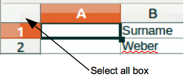
To select the entire sheet, click on the small box between the column headers and the row headers (Figure 13), use the key combination Ctrl+A, press Ctrl+Shift+Space, or go to Edit on the Menu bar and select Select All.
Figure 13: Select All box
You can select either one or multiple sheets in Calc. It can be advantageous to select multiple sheets, especially when you want to make changes to many sheets at once.
Click on the sheet tab for the sheet you want to select. The tab for the selected sheet becomes highlighted.
To select multiple contiguous sheets:
1) Click on the sheet tab for the first desired sheet.
2) While holding down the Shift key, click on the sheet tab for the last desired sheet.
3) All tabs between these two selections will be highlighted. Any actions that you perform will now affect all highlighted sheets.
To select multiple non-contiguous sheets:
1) Click on the sheet tab for the first desired sheet.
2) While holding down the Ctrl key, click on the sheet tabs for other desired sheets.
3) The selected tabs will be highlighted. Any actions that you perform will now affect all highlighted sheets.
Right-click a sheet tab and choose Select All Sheets in the context menu, or select Edit > Select > Select All Sheets on the Menu bar.
Tip
You can also select sheets using the Select Sheets dialog, accessed by selecting Edit > Select > Select Sheets on the Menu bar.
When you insert columns or rows, the cells take the formatting of the corresponding cells in the column to the left or the row above.
Using the Sheet menu:
1) Select a cell, column, or row where you want the new column or row inserted.
2) Go to Sheet on the Menu bar. For columns, select Sheet > Insert Columns and then select Columns Before or Columns After. For rows, select Sheet > Insert Rows and then select Rows Above or Rows Below.
Using the context menu:
1) Select a column or row where you want the new column or row inserted.
2) Right-click the column or row header.
3) Select Insert Columns Before / After or Insert Rows Above / Below in the context menu.
Multiple columns or rows can be inserted at once rather than inserting them one at a time.
1) Highlight the required number of columns or rows by holding down the left mouse button on the first one and then dragging across the required number of identifiers.
2) Proceed as for inserting a single column or row above. The number of columns or rows highlighted will be inserted.
To hide columns or rows from view, select the columns or rows to hide and do one of the following:
Right-click on the selected column or row headers and select Hide Columns / Rows.
From the Menu bar, select Format > Columns / Rows > Hide.
Tip
For a visible indication of hidden rows and columns, enable the option from the Menu bar, View > Hidden Row/Column Indicator.
To unhide columns or rows, select the entire sheet or the columns or rows around the columns or rows you wish to unhide and do one of the following:
Right-click on the selected column or row headers and select Show Columns / Rows.
From the Menu bar, select Format > Columns / Rows > Show.
To delete a single column or row, do one of the following:
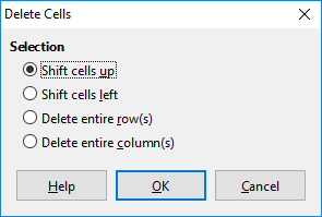
Select a cell in the column or row you want to delete, right-click and select Delete in the context menu, select Sheet > Delete Cells on the Menu bar, or press Ctrl+- to open the Delete Cells dialog (Figure 14). Select Delete entire column(s) or Delete entire row(s) and click OK.
Select a cell in the column or row you want to delete and select Sheet > Delete Columns or Sheet > Delete Rows.
Right-click the header of the column or row that you want to delete and select Delete Columns or Delete Rows in the context menu.
Figure 14: Delete Cells dialog
To delete multiple columns or rows, do one of the following:
Select a range of cells across the columns or rows you want to delete, right-click and select Delete in the context menu, select Sheet > Delete Cells on the Menu bar, or press Ctrl+- to open the Delete Cells dialog. Select Delete entire column(s) or Delete entire row(s) and click OK.
Select a range of cells across the columns or rows you want to delete and select Sheet > Delete Columns or Sheet > Delete Rows.
Highlight the required columns or rows by holding down the left mouse button on the header of the first one and then dragging across the required number of headers. Then right-click on one of the selected column or row headers and select Delete Columns or Delete Rows in the context menu.
1) Select the cell or cells you want to delete.
2) Select Sheet > Delete Cells, press Ctrl+-, or right-click on one of the selected cells and select Delete in the context menu.
3) Select the option you require from the Delete Cells dialog and click OK.
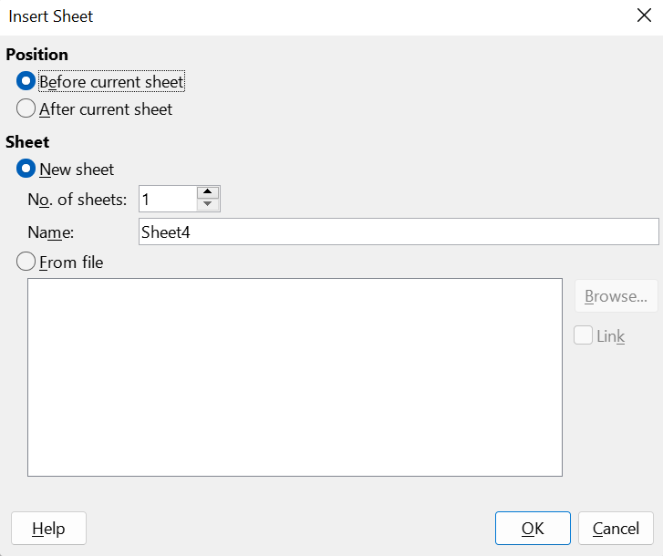
Click on the + symbol next to the sheet tabs to insert a new sheet after the last sheet in the spreadsheet without opening the Insert Sheet dialog. The following methods open the Insert Sheet dialog (Figure 15) where you can position the new sheet, create more than one sheet, name the new sheet, or select a sheet from a file.
Select the sheet where you want to insert a new sheet, then select Sheet > Insert Sheet on the Menu bar.
Right-click on the sheet tab where you want to insert a new sheet and select Insert Sheet in the context menu.
Click in the empty space at the end of the sheet tabs.
Right-click in the empty space at the end of the sheet tabs and select Insert Sheet from the context menu.
Figure 15: Insert Sheet dialog
You can move or copy sheets within the same spreadsheet by dragging and dropping or using the Move/Copy Sheet dialog (Figure 16). To move or copy a sheet into a different spreadsheet, use the Move/Copy Sheet dialog.
To move a sheet to a different position within the same spreadsheet, click on the sheet tab and drag it to its new position before releasing the mouse button.
To copy a sheet within the same spreadsheet, hold down the Ctrl key then click on the sheet tab and drag it to its new position before releasing the mouse button. The mouse pointer may change to include a plus sign depending on the setup of your operating system.
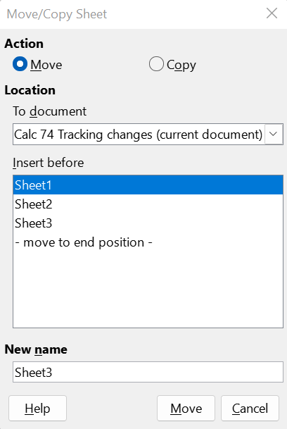
The Move/Copy Sheet dialog allows you to specify exactly whether you want the sheet in the same or a different spreadsheet, its position within the spreadsheet, and the sheet name when it is moved or copied.
1) In the current document, right-click on the sheet tab you wish to move or copy and select Move or Copy Sheet in the context menu, or go to Sheet > Move or Copy Sheet on the Menu bar.
2) Select Move to move the sheet or Copy to copy the sheet.
3) Select the spreadsheet where you want the sheet to be placed from the To document drop-down list. This can be the same spreadsheet, another spreadsheet that is already opened, or you can create a new spreadsheet.
4) Select the position in Insert before where you want to place the sheet.
5) Type a name in the New name text box if you want to rename the sheet when it is moved or copied. When copying, Calc suggests a default name (Sheet1_2, Sheet2_2, and so on).
6) Click Move or Copy to confirm the move or copy and close the dialog.
Figure 16: Move/Copy Sheet dialog
Caution
When you move or copy to another spreadsheet or to a new one, a conflict may occur if formulas are linked to sheets in the previous location.
To delete a single sheet, right-click on the sheet tab you want to delete and select Delete Sheet in the context menu, or go to Sheet > Delete Sheet on the Menu bar. Click Yes to confirm the deletion.
To delete multiple sheets, select the sheets (see “Selecting sheets” on page 1), then right-click one of the sheet tabs and select Delete Sheet in the context menu, or go to Sheet > Delete Sheet on the Menu bar. Click Yes to confirm the deletion.
Sometimes you may want to hide the contents of a sheet to preserve data from accidental editing or because its contents are not important to display.
To hide a sheet or many sheets, select the sheet or sheets as above, right-click to open the context menu, and select Hide Sheet.
To show hidden sheets, right-click any sheet tab and select Show Sheet in the context menu. A dialog will open with all hidden sheets listed. Select the desired sheets and then click OK.
Note
LibreOffice Calc does not let you hide the last visible sheet.
By default, the name for each new sheet added is SheetX, where X is the number of the next sheet to be added. While this works for a spreadsheet with only a few sheets, it can become difficult to identify sheets when a spreadsheet contains many sheets.
You can rename a sheet using one of the following methods:
Enter the name in the Name text box when you create the sheet using the Insert Sheet dialog (Figure 15 above).
Right-click on a sheet tab and select Rename Sheet in the context menu to open the Rename Sheet dialog
Select Sheet > Rename Sheet on the Menu bar to access the Rename Sheet dialog.
Double-click on a sheet tab to open the Rename Sheet dialog.
Note
Sheet names can contain almost any character. Some naming restrictions apply, the following characters are not allowed in sheet names: colon (:), back slash (\), forward slash (/), question mark (?), asterisk (*), left square bracket ([), or right square bracket (]). In addition a single quote (‘) cannot be used as the first or last character of the name.
Use the zoom function to show more or fewer cells in the window when you are working on a spreadsheet. For more about zoom, see Chapter 1, Introducing LibreOffice, in the Getting Started Guide.
Freezing is used to lock rows across the top of a spreadsheet or to lock columns on the left of a spreadsheet. Then, when moving around within a sheet, the cells in frozen rows and columns always remain in view.
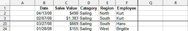
Figure 17 shows some frozen rows and columns. The heavier horizontal line between rows 3 and 23 and the heavier vertical line between columns F and Q indicate that rows 1 to 3 and columns A to F are frozen. The rows between 3 and 23 and the columns between F and Q have been scrolled off the page. To freeze rows or columns:
1) Click on the row header below the rows you want the freeze or click on the column header to the right of the columns where you want the freeze. To freeze both rows and columns, select the cell (not a row or column) that is below the row and to the right of the column that you want to freeze
2) Go to View on the Menu bar and select Freeze Rows and Columns. A heavier line appears between the rows or columns indicating where the freeze has been placed.
Figure 17: Frozen rows and columns
To unfreeze rows or columns, go to View on the Menu bar and click Freeze Rows and Columns to toggle it off. The heavier lines indicating freezing will disappear.
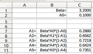
Another way to change the view is by splitting the screen displayed (also known as splitting the window). The screen can be split horizontally, vertically, or both, displaying up to four portions of the spreadsheet at the same time. An example of splitting the screen is shown in Figure 18 where a split is indicated by a gray line.
This could be useful for example, when a large spreadsheet has one cell with a number that is used by three formulas in other cells. Using the split-screen technique, the cell containing the number can be positioned in one section of the view and the cells with formulas can be seen in the other sections. This makes it easy to see how changing the number in one cell affects each of the formulas.
Figure 18: Split screen example
There are two ways to split a screen horizontally or vertically:
Method One:
1) Click on the row header below the rows where you want to split the screen horizontally or click on the column header to the right of the columns where you want to split the screen vertically.
2) Go to View on the Menu bar and select Split Window or right-click and choose Split Window in the context menu. A thick line appears between the rows or columns indicating where the split has been placed. An example of a split line is shown below Row 2 in Figure 18.
Method Two:
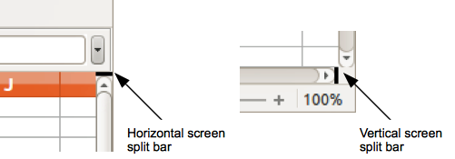
For a horizontal split, click on the thick black line at the top of the vertical scroll bar (Figure 19) and drag the split line below the row where you want the horizontal split positioned.
Similarly, for a vertical split, click on the thick black line at the right of the horizontal scroll bar (Figure 19) and drag the split line to the right of the column where you want the vertical split positioned.
Figure 19: Split screen bars
Position both the black horizontal and the black vertical lines as described above and as shown in Figure 19.
1) Click the cell that is immediately below the rows where you want to split the screen horizontally and immediately to the right of the columns where you want to split the screen vertically.
2) Go to View on the Menu bar and select Split Window. Thick lines appear between the rows and columns indicating where the splits have been placed.
To remove a split view, do any of the following:
Double-click on each split line in turn.
Click on and drag the split lines back to their places at the ends of the scroll bars.
Go to View on the Menu bar and click Split Window to toggle it off.
Right-click on a column or row heading and click Split Window in the context menu to toggle it off.
The Navigator (Figure 20) is available in all LibreOffice modules. It provides tools and methods to move quickly through a spreadsheet and find specific items.
The Navigator categorizes and groups spreadsheet objects which you can click on to move quickly to that object. If an indicator (plus sign or triangle, dependent on computer setup) appears next to a category, at least one object in this category exists. To open a category and see the list of items, click on the indicator. When a category is showing the list of objects in it, double-click on an object to jump directly to that object’s location in the spreadsheet.
To open the Navigator, do one of the following:
Press the F5 key.
Select View > Navigator on the Menu bar.
Click the Navigator icon on the Tab panel of the Sidebar.
Figure 20: Navigator dialog in Calc
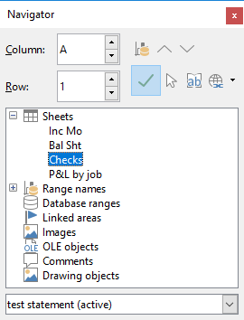
The controls and tools available in the Navigator are as follows:
Column – type a column letter and press the Enter key to reposition the cell cursor to the specified column in the same row.
Row – type a row number and press the Enter key to reposition the cell cursor to the specified row in the same column.
Data Range – highlights the data range containing the cell in which the cursor currently lies. Calc checks the content of adjacent cells and determines the data range automatically. The data range can comprise one cell if there is no data in adjacent cells.
Start – moves the cursor to the cell at the beginning of the current data range, which you can highlight using the Data Range icon.
End – moves the cursor to the cell at the end of the current data range, which you can highlight using the Data Range icon.
Contents – toggles on / off the display of the contents view in the lower part of the Navigator dialog, to temporarily reduce its size. There is no equivalent control needed on the Navigator deck of the Sidebar.
Toggle – toggles the contents view. Only the selected category and its objects are displayed. Click the icon again to restore all elements for viewing.
Scenarios – displays all available scenarios. See Chapter 10, Data Analysis, for more information about scenarios. Double-click a name to apply that scenario and the result is shown in the sheet. If the Navigator displays scenarios, you can access the following commands when you right-click a scenario entry:
Delete – deletes the selected scenario.
Properties – opens the Edit Scenario dialog, where you can edit the scenario properties.
Drag Mode – opens a submenu for selecting which action is performed when dragging and dropping an object from the Navigator into a document. Depending on the mode you select, the icon indicates whether a hyperlink, a link, or a copy is created.
Insert as Hyperlink – hyperlinks the entire item.
Insert as Link – links the copied item to the original item so that when the original item is changed, that change will be reflected in the current document.
Insert as Copy – inserts a copy of the selected item.
Tip
Ranges, scenarios, pictures, and other objects are much easier to find if you have given them informative names when creating them, instead of keeping the default Calc names, for example Scenario 1, Image 1, Image 2, Object 1, and so on. These default names may not correspond to the position of the object in the document.
To open the Properties dialog for a document, go to File > Properties on the Menu bar. The Properties dialog provides information about the spreadsheet and allows you to set some of its properties. The dialog is shown in Figure 21 and its tabs are described below.
Figure 21: Properties dialog, General tab
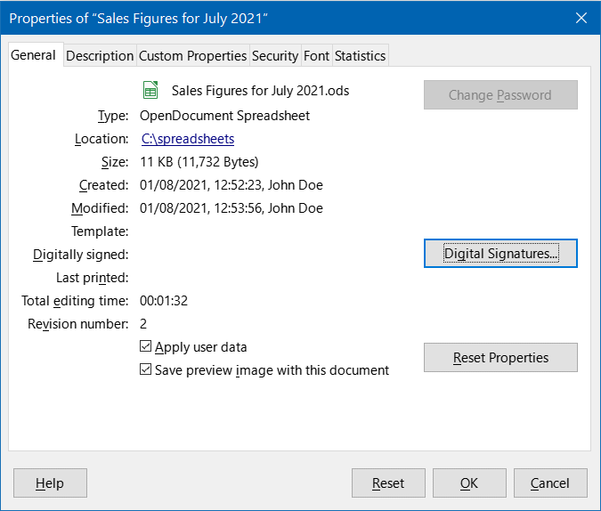
Contains basic information about the current file.
The text at the top of the dialog displays the file name.
Change Password – opens a dialog to change the password. It is only active if a password has been set for the file.
Type – displays the file type of the current document.
Location – displays the path and the name of the directory where the file is stored. In the case of a local file, this is a clickable link that opens the file browser to view the folder. For remote content (shown as, for example, http://...), the link opens a web browser.
Size – displays the size of the current document in bytes.
Created – displays the date, time, and author when the file was first opened.
Modified – displays the date, time, and author when the file was last saved in a LibreOffice file format.
Template – displays the template that was used to create the file, if applicable.
Digitally signed – displays the date and time when the file was last signed as well as the name of the author who signed the document.
Digital Signatures – opens the Digital Signatures dialog where you can manage digital signatures for the current document.
Last printed – displays the date, time, and user name when the file was last printed.
Total editing time – displays the amount of time that the file has been open for editing since the file was created. The editing time is updated when you save the file.
Revision number – displays the number of times that the file has been saved.
Apply user data – saves the full name of the user with the file. You can edit the name by going to Tools > Options > LibreOffice > User Data on the Menu bar.
Save preview image with this document – saves a thumbnail.png inside the document. These images may be used by a file manager under certain conditions.
Reset Properties – resets the editing time to zero, the creation date to the current date and time, and the version number to 1. The modification and printing dates are also deleted.
Contains optional editable descriptive information about the spreadsheet.
Title – enter a title for the spreadsheet.
Subject – enter a subject for the spreadsheet. You can use a subject to group documents with similar content.
Keywords – enter the words that you want to use to index the content of the spreadsheet. Keywords must be separated by commas. A keyword can contain white space characters or semicolons.
Comments – enter comments to help identify the spreadsheet.
Use this page to assign custom information fields to the spreadsheet. In a new spreadsheet, this page may be blank. If the new spreadsheet is based on a template, this page may contain fields. You can change the name, type, and contents of each row. The information in the fields will be exported as metadata to other file formats.
Click Add Property to add a new custom property. Use the red “X” button at the end of an entry to delete the custom property.
Only relevant for spreadsheets stored on remote servers. See the Help or the Getting Started Guide for more information.
Enables two password-protected security options.
Open file read-only – select to allow this document to be opened only in read-only mode. This file sharing option protects the document against accidental changes. It is still possible to edit a copy of the document and save that copy with the same name as the original.
Record changes – select to require that all changes be recorded. To protect the recording state with a password, click Protect and enter a password. This is similar to Edit > Track Changes > Record on the Menu bar. However, while other users of this document can apply their changes, they cannot disable change recording without knowing the password.
Protect or Unprotect – protects the change recording state with a password. If change recording is protected for the current document, the button is named Unprotect. Click Unprotect to disable the protection.
When Embed fonts in the document is selected, any fonts used in the spreadsheet will be embedded into the document when it is saved. This may be useful if you are creating a PDF of the spreadsheet and want to control how it will look on other computer systems.
Only embed fonts that are used in documents – If fonts have been defined for the spreadsheet (for example, in the template), but have not been used, select this option to not embed them.
Font scripts to embed – You can choose which types of fonts are embedded: Latin, Asian, Complex. See the Getting Started Guide for more information.
Displays statistics for the current file: the number of sheets, cells, pages, and formula groups.