Calc Guide 7.4
Chapter 8
Using Formulas and Functions
This document is Copyright © 2022 by the LibreOffice Documentation Team. Contributors are listed below. You may distribute it and/or modify it under the terms of either the GNU General Public License (https://www.gnu.org/licenses/gpl.html), version 3 or later, or the Creative Commons Attribution License (https://creativecommons.org/licenses/by/4.0/), version 4.0 or later.
All trademarks within this guide belong to their legitimate owners.
|
Skip Masonsmith |
Kees Kriek |
|
|
Barbara Duprey |
Jean Hollis Weber |
John A Smith |
|
Olivier Hallot |
Kees Kriek |
Steve Fanning |
|
Leo Moons |
Gordon Bates |
Felipe Viggiano |
|
Rachel Kartch |
|
|
Please direct any comments or suggestions about this document to the Documentation Team’s forum at https://community.documentfoundation.org/c/documentation/loguides/ (registration is required) or send an email to: loguides@community.documentfoundation.org.
Note
Everything you post to a forum, including your email address and any other personal information that is written in the message, is publicly archived and cannot be deleted. E-mails sent to the forum are moderated.
Published October 2022. Based on LibreOffice 7.4 Community.
Other versions of LibreOffice may differ in appearance and functionality.
Some keystrokes and menu items are different on macOS from those used in Windows and Linux. The table below gives some common substitutions for the instructions in this document. For a more detailed list, see the application Help and Appendix A (Keyboard Shortcuts) to this guide.
|
Windows or Linux |
macOS equivalent |
Effect |
|
Tools > Options menu selection |
LibreOffice > Preferences |
Access setup options |
|
Right-click |
Control+click and/or right-click depending on computer setup |
Opens a context menu |
|
Ctrl (Control) |
⌘ (Command) |
Used with other keys |
|
F11 |
⌘+T |
Opens the Styles deck in the Sidebar |
In previous chapters, we have been entering one of two basic types of data into each cell: numbers and text. However, we will not always know what the contents should be. Often the contents of one cell depends on the contents of other cells. To handle this situation, we use a third type of data: the formula. Formulas are equations using numbers and variables to get a result. In a spreadsheet, the variables are cell locations that hold the data needed for the equation to be completed.
A function is a predefined calculation entered in a cell to help you analyze or manipulate data. All you have to do is add the arguments, and the calculation is made automatically. Functions help you create the formulas needed to get the results that you are looking for.
If you are setting up more than a simple one-sheet system in Calc, it is worth planning ahead a little. Make sure to:
Avoid typing fixed values into formulas
Include documentation (notes and comments) describing what the system does, including what input is required and where the formulas come from (if not created from scratch)
Incorporate a system of error-checking of formulas to verify that the formulas do what is intended
Many users set up long and complex formulas with fixed values typed directly into the formula.
For example, conversion from one currency to another requires knowledge of the current conversion rate. If you input a formula in cell C1 of =0.75*B1 (for example to calculate the value in Euros of the USD dollar amount in cell B1), you will have to edit the formula when the exchange rate changes from 0.75 to some other value. It is much easier to set up an input cell with the exchange rate and reference that cell in any formula needing the exchange rate. What-if type calculations are also simplified: what if the exchange rate varies from 0.75 to 0.70 or 0.80? No formula editing is needed and it is clear what rate is used in the calculations. Breaking complex formulas down into more manageable parts, described below, also helps to minimize errors and aid troubleshooting.
Lack of documentation is a very common point of failure. Many users prepare a simple sheet which then develops into something much more complicated over time. Without documentation, the original purpose and methodology is often unclear and difficult to decipher. In this case it is usually easier to start again from the beginning, wasting the work done previously. If you insert comments in cells, and use labels and headings, a spreadsheet can later be easily modified by you or others and much time and effort will be saved.
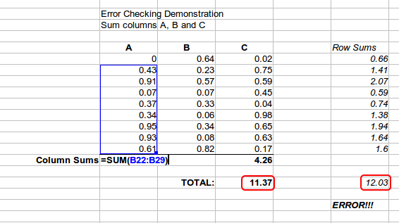
Adding up columns of data or selections of cells from a sheet often results in errors due to omitting cells, wrongly specifying a range, or double-counting cells. It is useful to institute checks in your spreadsheets. For example, set up a spreadsheet to calculate columns of figures, and use the function SUM to calculate the individual column totals. You can check the result by including (in a non-printing column) a set of row totals and adding these together. The two values—row total and column total—must agree. If they do not, you have an error somewhere.
You can even set up a formula to calculate the difference between the two totals and report an error in case a non-zero result is returned (see Figure 1).
Figure 1: Error checking of formulas
You can enter formulas in two ways. One method is to use the Function Wizard or the equivalent facilities in the Functions deck of the Sidebar. The second method is to type directly into the cell or into the Input line. A formula must begin with an = symbol. When typing directly, you normally need to start a formula with =. However, if your formula begins with a + or – (for example -2*A1), then Calc automatically adds the = symbol. An = is not added if you simply enter a positive or negative number (such as -2 or +3). Starting with anything else causes your intended formula to be treated as if it were text.
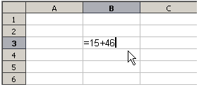
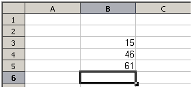
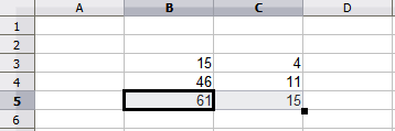
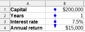
Each cell in the sheet can be used as a data holder or a place for data calculations. To enter data, simply type in the cell and move to the next cell or press Enter. With formulas, the equals sign indicates that the cell will be used for a calculation. An example of a mathematical calculation like 15 + 46 is shown in Figure 2.
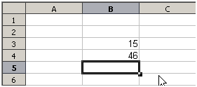
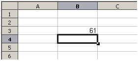
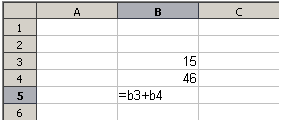
While the calculation on the left used only one cell, the real power is shown on the right where the data is placed in cells and the calculation is performed using references to the cells. In this case, cells B3 and B4 were the data holders, with B5 the cell where the calculation was performed. Notice that the formula was shown as =B3+B4. The plus sign indicates that the contents of cells B3 and B4 are to be added together and then have the result in the cell holding the formula. All formulas build upon this concept. Other ways of using formulas are shown in Table 1.
These cell references allow formulas to use data from anywhere in the sheet being worked on, or from any other sheet in the document that is opened. If the data needed was in different sheets, they would be referenced by referring to the name of the sheet, for example =$Sheet2.B12+$Sheet3.A11.
Note
To enter the = symbol for a purpose other than creating a formula as described in this chapter, type an apostrophe or single quotation mark before the =. For example, in the entry '= means different things to different people, Calc treats everything after the single quotation mark—including the = sign—as text.
|
Simple Calculation in 1 Cell |
Calculation by Reference |
|
|
|
|
|
|
|
|
|
Figure 2: A simple calculation
Table 1: Common ways to use formulas
|
Formula |
Description |
|
=A1+10 |
Displays the contents of cell A1 plus 10. |
|
=A1*16% |
Displays 16% of the contents of A1. |
|
=A1*A2 |
Displays the result of multiplying the contents of A1 and A2. |
|
=ROUND(A1,1) |
Displays the contents of cell A1 rounded to one decimal place. |
|
=EFFECT(5%,12) |
Calculates the effective interest for 5% annual nominal interest with 12 payments a year. |
|
=B8-SUM(B10:B14) |
Calculates B8 minus the sum of the cells B10 to B14. |
|
=SUM(B8,SUM(B10:B14)) |
Calculates the sum of cells B10 to B14 and adds the value to B8. |
|
=SUM(B1:B1048576) |
Sums all numbers in column B. |
|
=AVERAGE(BloodSugar) |
Displays the average of a named range defined under the name BloodSugar. It is possible to establish ranges for inclusion by naming them using Sheet > Named Ranges and Expressions > Define, for example BloodSugar representing a range such as B3:B10. |
|
=IF(C31>140, “HIGH”, “OK”) |
Logical functions can also be performed as represented by the IF statement which results in a conditional response based upon the data in the identified cell. In this example, if the contents of C31 is greater than 140, then HIGH is displayed, otherwise OK is displayed. |
You can use the following operator types in Calc: arithmetic, comparative, text, and reference.
The addition, subtraction, multiplication, and division operators return numerical results. The negation and percent operators identify a characteristic of the number found in the cell, for example -37. The example for exponentiation illustrates how to enter a number that is being multiplied by itself a certain number of times, for example 2^3 = 2*2*2.
Table 2: Arithmetic operators
|
Operator |
Name |
Example |
|
+ (Plus) |
Addition |
=1+1 |
|
– (Minus) |
Subtraction |
=2–1 |
|
– (Minus) |
Negation |
–5 |
|
* (Asterisk) |
Multiplication |
=2*2 |
|
/ (Slash) |
Division |
=10/5 |
|
% (Percent) |
Percent |
15% |
|
^ (Caret) |
Exponentiation |
=2^3 |
Comparative operators are found in formulas that use the IF function and return either a true or false answer; for example, =IF(B6>G12, 127, 0) which, loosely translated, means if the contents of cell B6 are greater than the contents of cell G12, then return the number 127, otherwise return the number 0.
A direct answer of TRUE or FALSE can be obtained by entering a formula such as =B6>B12. If the numbers found in the referenced cells are accurately represented, the answer TRUE is returned, otherwise FALSE is returned.
Table 3: Comparative operators
|
Operator |
Name |
Example |
Result (A=4, B=5) |
|
= |
Equal |
A1=B1 |
FALSE |
|
> |
Greater than |
A1>B1 |
FALSE |
|
< |
Less than |
A1<B1 |
TRUE |
|
>= |
Greater than or equal to |
A1>=B1 |
FALSE |
|
<= |
Less than or equal to |
A1<=B1 |
TRUE |
|
<> |
Inequality |
A1<>B1 |
TRUE |
If cell A1 contains the numerical value 4 and cell B1 contains the numerical value 5, the above examples would yield results of FALSE, FALSE, TRUE, FALSE, TRUE, and TRUE.
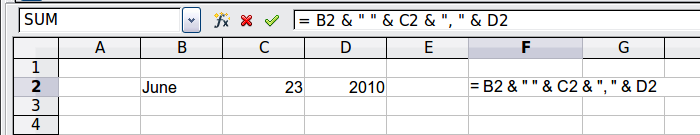
It is common for users to place text in spreadsheets. To provide for variability in what and how this type of data is displayed, text can be joined together in pieces coming from different places on the spreadsheet. Figure 3 shows an example.
|
|
|
|
|
Figure 3: Text concatenation |
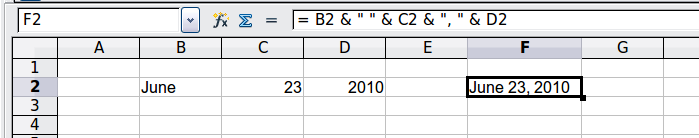
In this example, specific pieces of the text were found in three different cells. To join these segments together, the formula also adds required spaces and punctuation enclosed within quotation marks, resulting in a formula of =B2 & “ ” & C2 & “, ” & D2. The result is the concatenation into a date formatted in a particular sequence.
Calc has a CONCATENATE function which performs the same operation.
An individual cell is identified by the column identifier (letter) located along the top of the columns and a row identifier (number) found along the left-hand side of the spreadsheet. On spreadsheets read from left to right, the reference for the upper left cell is A1.
Thus in its simplest form a reference refers to a single cell, but references can also refer to a rectangle or cuboid range, or a reference in a list of references. To build such references you need reference operators.
The range operator is written as a colon. An expression using the range operator has the following syntax:
reference upper left : reference lower right
The range operator builds a reference to the smallest range including both the cells referenced with the left reference and the cells referenced with the right reference.
In the upper left corner of Figure 4 the reference A1:D12 is shown, corresponding to the cells included in the drag operation with the mouse to highlight the range.
Figure 4: Reference operator for a range
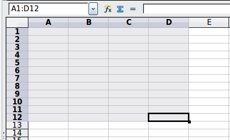
Table 4: Reference range operator examples
|
Example |
Description |
|
A2:B4 |
Reference to a rectangle range with 6 cells, 2 column width × 3 row height. When you click on the reference in the formula in the input line, a border indicates the rectangle. |
|
(A2:B4):C9 |
Reference to a rectangle range with cell A2 top left and cell C9 bottom right. So the range contains 24 cells, 3 column width × 8 row height. This method of addressing extends the initial range from A2:B4 to A2:C9. |
|
Sheet1.A3:Sheet3.D4 |
Reference to a cuboid range with 24 cells, 4 column width × 2 row height × 3 sheets depth. (Assumes that sheets Sheet1, Sheet2, and Sheet3 appear in that order on the Sheet tabs area.) |
|
B:B |
Reference to all cells of column B. |
|
A:D |
Reference to all cells of columns A to D. |
|
20:20 |
Reference to all cells of row 20. |
|
1:20 |
Reference to all cell of rows 1 to 20. |
When you enter B4:A2, B2:A4, or A4:B2 directly, Calc will turn it to A2:B4. So the left top cell of the range is left of the colon and the bottom right cell is right of the colon. But if you name the cell B4 for example with _start and A2 with _end, you can use _start:_end without any error. For more information on naming cells, see “Named ranges” on page 1.
The concatenation operator is written as a tilde. An expression using the concatenation operator has the following syntax:
reference left ~ reference right
The result of such an expression is a reference list, which is an ordered list of references. Some functions can take a reference list as an argument, SUM, MAX, or INDEX for example.
The reference concatenation is sometimes called 'union'. But it is not the union of the two sets 'reference left' and 'reference right' as normally understood in set theory. COUNT(A1:C3~B2:D2) returns 12 (=9+3), but it has only 10 cells when considered as the union of the two sets of cells.
Notice that SUM(A1:C3,B2:D2) is different from SUM(A1:C3~B2:D2) although they give the same result. The first is a function call with 2 parameters, each of them is reference to a range. The second is a function call with 1 parameter, which is a reference list.
The reference concatenation also applies to whole rows and whole columns. For example SUM(A:B~D:D) is the sum of all cells in columns A and B and the column D.
The intersection operator is written as an exclamation mark. An expression using the intersection operator has the following syntax:
reference left ! reference right
If the references refer to single ranges, the result is a reference to a single range, containing all cells, which are both in the left reference and in the right reference.
If the references are reference lists, then each list item from the left is intersected with each one from the right and these results are concatenated to a reference list. The order is to first intersect the first item from the left with all items from the right, then intersect the second item from the left with all items from the right, and so on.
Examples
A2:B4 ! B3:D6
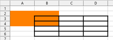
This results in a reference to the range B3:B4, because these cells are inside A2:B4 and inside B3:D6. This is illustrated in Figure 5, in which the cells in the range A2:B4 have orange backgrounds and the cells in the range B3:D6 have thick black borders. The cells that have both an orange background and a thick black border (B3:B4) form the intersection of the two ranges.
Figure 5: Simple example of reference intersection operator
(A2:B4~B1:C2) ! (B2:C6~C1:D3)
First the intersections A2:B4!B2:C6, A2:B4!C1:D3, B1:C2!B2:C6, and B1:C2!C1:D3 are calculated. This results in B2:B4, empty, B2:C2, and C1:C2. Then these results are concatenated, dropping empty parts. So the final result is the reference list B2:B4 ~ B2:C2 ~ C1:C2.
A:B ! 10:10
Calculates the intersection of columns A and B with line 10, thus selecting A10 and B10.
You can use the intersection operator to refer to a cell in a cross tabulation in an understandable way. If you have columns labeled 'Temperature' and 'Precipitation' and the rows labeled 'January', 'February', 'March', and so on, then the following expression
'February' ! 'Temperature'
will reference the cell containing the temperature in February.
The intersection operator (!) has a higher precedence than the concatenation operator (~), but do not rely on precedence.
Tip
Always put in parentheses the part that is to be calculated first.
References are the way that we refer to the location of a particular cell in Calc and can be either relative (to the current cell) or absolute (a fixed amount).
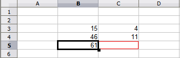
An example of a relative reference will illustrate the difference between a relative reference and absolute reference using the spreadsheet from Figure 6.
1) Type the numbers 4 and 11 into cells C3 and C4 respectively of that spreadsheet.
2) Copy the formula in cell B5 (=B3+B4) to cell C5. You can do this by using a simple copy and paste or click and drag B5 to C5 as shown below. The formula in B5 calculates the sum of values in the two cells B3 and B4.
3) Click in cell C5. The formula bar shows =C3+C4 rather than =B3+B4 and the value in C5 is 15, the sum of 4 and 11 which are the values in C3 and C4.
In cell B5 the references to cells B3 and B4 are relative references. This means that Calc interprets the formula in B5, applies it to the cells in the B column, and puts the result in the cell holding the formula. When you copied the formula to another cell, the same procedure was used to calculate the value to put in that cell. This time the formula in cell C5 referred to cells C3 and C4.
You can think of a relative address as a pair of offsets to the current cell. Cell B1 is 1 column to the left of cell C5 and 4 rows above. The address could be written as R[-4]C[-1]. In fact earlier spreadsheets allowed this notation method to be used in formulas.
Whenever you copy this formula from cell B5 to another cell, the result will always be the sum of the two numbers taken from the two cells one and two rows above the cell containing the formula.
Relative addressing is the default method of referring to addresses in Calc.
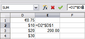
You may want to multiply a column of numbers by a fixed amount. A column of figures might show amounts in US Dollars. To convert these amounts to Euros it is necessary to multiply each dollar amount by the exchange rate. $US10.00 would be multiplied by 0.75 to convert to Euros, in this case Eur7.50. The following example shows how to input an exchange rate and use that rate to convert amounts in a column from USD to Euros.
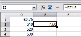
1) Input the exchange rate Eur:USD (0.75) in cell D1. Enter amounts (in USD) into cells D2, D3 and D4, for example 10, 20, and 30.
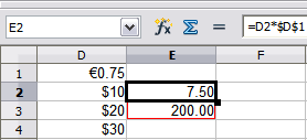
2) In cell E2 type the formula =D2*D1. The result is 7.5, correctly shown.
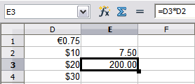
3) Copy the formula in cell E2 to cell E3. The result is 200, clearly wrong! Calc has copied the formula using relative addressing: the formula in E3 is =D3*D2 and not what we want, which is =D3*D1.
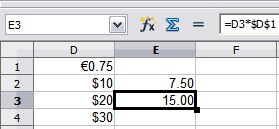
4) In cell E2 edit the formula to be =D2*$D$1. Copy it to cells E3 and E4. The results are now 15 and 22.5 which are correct.
The $ signs before the D and the 1 convert the reference to cell D1 from relative to absolute or fixed. If the formula is copied to another cell the second part will always show $D$1. The interpretation of this formula is “take the value in the cell one column to the left in the same row and multiply it by the value in cell D1”.
|
|
|
|
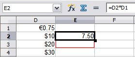
Enter the conversion formula into E2, which will show the correct result, then copy it to E3. |
|
|
|
|
|
E3 result is clearly wrong; change the formula in E2 to use absolute reference. |
|
|
|
|
|
Copy the correct formula from E2 to E3 to get the correct answer. |
|
|
Figure 7: Absolute references |
|
Cell references can be shown in four ways, listed in Table 5.
Table 5: Cell reference types
|
Reference |
Explanation |
|
D1 |
Relative, from cell E3 it is the cell one column to the left and two rows above |
|
$D$1 |
Absolute, it is the cell D1 |
|
$D1 |
Partially absolute, from cell E3 it is the cell in column D and two rows above |
|
D$1 |
Partially absolute, from cell E3 it is the cell one column to the left and in row 1 |
Tip
To change references in formulas, highlight the cell and press F4 to cycle through the four types of references. To cycle only part of the formula select the cells in the formula bar and cycle with F4. Selecting the menu option Sheet > Cycle Cell Reference Types is equivalent to pressing the F4 shortcut.
Knowledge of the use of relative and absolute references is essential if you want to copy and paste formulas and to link spreadsheets.
Cells and cell ranges can have a name assigned to them. Naming cells and ranges enhances formula readability and document maintenance. A simple example would be naming a range of cells B1:B10 as “Weight” and sum all weights. The formula is =SUM(B1:B10). When the range B1:B10 is named as Weight, you can transform the formula to =SUM(Weight). The advantage is clear in terms of readability of the formulas.
Another advantage is that all formulas that have the named range as argument are updated when the named range changes location or size. For example, if the range Weight is now in cells P10:P30, you do not need to review all the formulas that have Weight as an argument; you only need to update the named range Weight with the new size and location.
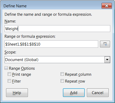
To define a named cell or range select the cell or range and use menu Sheet > Named Ranges and Expressions > Define. The dialog in Figure 8 appears with the selected range and you define the name and scope of the named range.
Figure 8: Define Name dialog
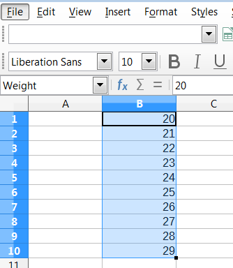
You can also define a named range directly in the sheet by selecting the range and typing its name in the Name Box at the left of the Formula Bar (Figure 9).
Figure 9: Inserting name in the range box to define a named range
To quickly access a named range, select the named range in the Name Box drop-down above. The named range is shown on the screen and selected.
Figure 10: Manage Names dialog
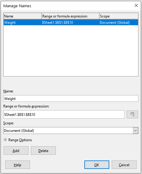
To modify a named range, use the Manage Names dialog (Figure 10). This dialog is accessed by selecting Sheet > Named Ranges and Expressions > Manage on the Menu bar or pressing Ctrl+F3.
You also can give a long or complex formula a name. To name a formula, open the Define Name dialog (Figure 8) and enter the formula expression in the Range or formula expression box. Name the expression and click Add.
As an example, suppose you need to compute in cells C1 to C10 the circumference of a set of circles and you are given their radius in B1 to B10. Define a named expression CIRCUMFERENCE, with expression =2*PI()*B1 and click Add to close the dialog. In cell C1, type =CIRCUMFERENCE and press Enter. The formula is applied to cell C1. Copy cell C1 and paste in the remaining cells from C2 to C10 and you have the circumferences of all the circles. All cells in the range C1:C10 have the expression =CIRCUMFERENCE.
Note that the named expression uses the same rules for cell addressing, that is, absolute and relative references.
Order of calculation refers to the sequence in which numerical operations are performed and the Wikipedia article at https://en.wikipedia.org/wiki/Order_of_operations provides useful general background information. Division and multiplication are performed before addition or subtraction. There is a common tendency to expect calculations to be made from left to right as the equation would be read in English. Calc evaluates the entire formula, then based upon programming precedence, breaks the formula down executing multiplication and division operations before other operations. Therefore, when creating formulas you should test your formula to make sure that the expected and correct result is being obtained. Following is an example of the order of calculation in operation.
Table 6: Order of calculation
|
Left To Right Calculation |
Ordered Calculation |
|
1+3*2+3 = 11 1+3 = 4, then 4x2 = 8, then 8+3 = 11 |
=1+3*2+3 result 10 3*2 = 6, then 1+6+3 = 10 |
|
Another possible intention could be: 1+3*2+3 = 20 1+3 = 4, then 2+3 = 5, then 4x5=20 |
The program resolves the multiplication of 3 x 2 before dealing with the numbers being added. |
If you intend for the result to be either of the two possible solutions on the left, order the formula as:
|
((1+3) * 2)+3 = 11 |
(1+3) * (2+3) = 20 |
Note
Use parentheses to group operations in the order you intend; for example, =B4+G12*C4/M12 might become =((B4+G12)*C4)/M12.
Another powerful feature of Calc is the ability to link data through several sheets. The naming of sheets can be helpful to identify where specific data may be found. A name such as Payroll or Boise Sales is much more meaningful than Sheet1. The function named SHEET() returns the sheet number (position) in the collection of sheets. There may be several sheets in each document and they may be numbered from the left: Sheet1, Sheet2, and so forth. If you drag the sheets around to different locations among the tabs, the function returns the number referring to the current position of this sheet. In a new instance of Calc, the default is a single sheet.
For example, if the formula =SHEET() is put into A1 on Sheet 1 it returns the value 1. If you drag Sheet 1 to be positioned between sheets 2 and 3 then the value changes to 2; it is now the second sheet in the order.
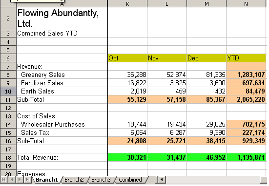
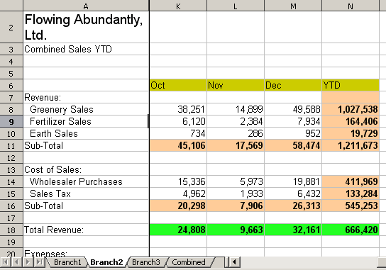
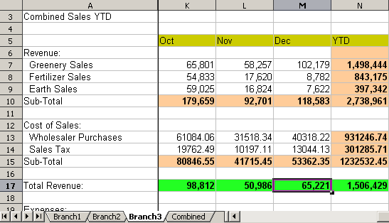
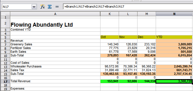
An example of calculations obtaining data from other work can be seen in a business setting where a business combines revenues and costs of each of its branch operations into a single combined sheet. See the four parts of Figure 11 below.
|
|
|
|
|
Sheet containing data for Branch 2. |
|
|
Sheet containing data for Branch 3. |
|
|
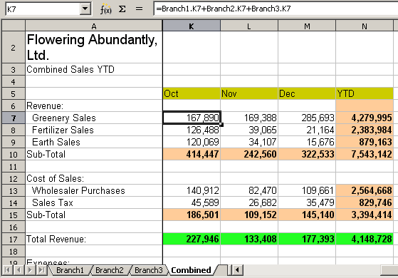
Sheet containing combined data for all branches. |
|
Figure 11: Combining data from several sheets into a single sheet |
|
The sheets have been set up with identical structures. The easiest way to do this is to open a new spreadsheet, set up the first branch sheet, input data, format cells, and prepare the formulas for the various sums of rows and columns. After that, create copies from the first sheet as follows:
1) On the sheet tab, right-click and select Rename Sheet. Type Branch1. Right-click on the tab again and select Move or Copy Sheet.
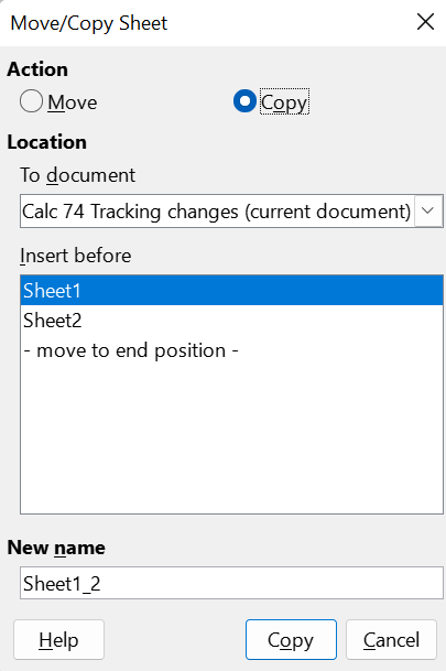
2) In the Move/Copy Sheet dialog (Figure 12), select the Copy option (automatically selected if there is only one sheet in the spreadsheet) and select -move to end position- in the Insert before area. Change the entry in New name to Branch2. Click Copy. Repeat to produce the Branch3 and Combined sheets.
Figure 12: Copying a sheet
3) Enter the data for Branch 2 and Branch 3 into the respective sheets. Each sheet stands alone and reports the results for the individual branches.
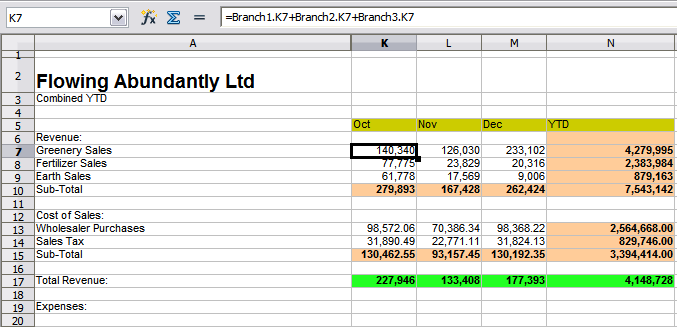
4) In the Combined sheet, click on cell K7. Type =, click on the tab Branch1, click on cell K7, press +, repeat for sheets Branch2 and Branch3, and press Enter. You now have a formula in cell K7 which adds the revenue from greenery sales for the three branches.
Figure 13: Combined sheet showing linking between branch sheets
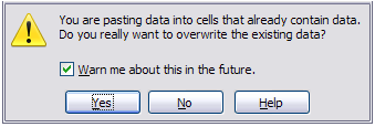
5) Copy the formula, highlight the range K7:N17, click Edit > Paste Special > Paste Special on the Menu bar, or right-click and select Paste Special > Paste Special in the context menu, or press Ctrl+Shift+V. Uncheck the All and Formats options in the Paste area of the dialog, check all other options in that area, and click OK. You will see the following message:
Figure 14: Linking sheets: pasting a formula to a cell range
6) Click Yes. You have now copied the formulas into each cell while maintaining the format set up in the original sheet. Of course, in this example you would have to tidy up the sheet by removing the zeros in the non-formatted rows.
Figure 15: Linking sheets: Copy / Paste Special from K7:N17
The Function Wizard can also be used to accomplish the linking. Use of this wizard is described in detail in “Using the Function Wizard” on page 1.
Calc includes over 500 functions to help you analyze and reference data. Many of these functions are for use with numbers, but others are used with dates and times or even text. A function may be as simple as adding two numbers together or finding the average of a list of numbers, or it may be as complex as calculating the standard deviation of a sample or a hyperbolic tangent of a number.
Typically, the name of a function is an abbreviated description of what the function does. For instance, the FV function gives the future value of an investment, while BIN2HEX converts a binary number to a hexadecimal number. In Calc, functions can be entered either in upper, lower or mixed cases.
A few basic functions are somewhat similar to operators. Examples:
|
+ |
This operator adds two numbers together for a result. SUM() on the other hand adds groups of contiguous ranges of numbers together. |
|
* |
This operator multiplies two numbers together for a result. PRODUCT() does the same for multiplying that SUM() does for adding. |
Each function has a number of arguments used in the calculations. These arguments may or may not have their own name. Your task is to enter the arguments needed to run the function. In some cases, the arguments have predefined choices, and you may need to refer to the text on the Function Wizard and the Functions deck, or the Help, to understand them. More often, however, an argument is a value that you enter manually, or one already entered in a cell or range of cells in the spreadsheet. In Calc, you can enter values from other cells by typing in their name or range, or—unlike the case in some spreadsheets—by selecting cells with the mouse. If the values in the cells change, then the result of the function is automatically updated.
Tip
You can find more details about each of the available functions in the Calc Functions area of The Document Foundation Wiki at https://wiki.documentfoundation.org/Documentation/Calc_Functions. These wiki pages are a recent addition to the available documentation and are continuously undergoing improvement.
For many functions, Calc follows the OpenFormula standard defined in Part 2 (Recalculated Formula (OpenFormula) Format) of the Open Document Format for Office Applications (OpenDocument) Version 1.2. This standard can be accessed at the OASIS website (https://www.oasis-open.org/) or the ISO website (https://www.iso.org/standard/66375.html). Calc’s general support for OpenFormula leads to a level of inherent compatibility with the function set of any other spreadsheet application that follows the same standard. (There are some functions within Calc that are not in accordance with OpenFormula but many of these are included specifically to improve the exchange of files between Calc and Microsoft Excel.)
In order to improve interoperability, Calc is able to open spreadsheets created by many different applications and to save them in many different formats. In the case of Microsoft Office, it is extremely straightforward to exchange spreadsheet files between the two applications. When Calc opens a Microsoft Excel spreadsheet, it automatically takes steps to avoid incompatibilities that might otherwise be encountered with certain functions.
For example, when Calc opens an Excel file that contains calls to Excel’s CEILING function, these are automatically converted to reference Calc’s CEILING.XCL function. Similarly when Calc saves a spreadsheet to Microsoft Excel format, it automatically takes steps to avoid potential incompatibilities. An example of this occurs when Calc saves a spreadsheet containing calls to its FLOOR function, as these are automatically converted to reference Excel’s FLOOR.MATH function.
The Document Foundation’s wiki provides a comparison of the features of LibreOffice and Microsoft Office, see https://wiki.documentfoundation.org/Feature_Comparison:_LibreOffice_-_Microsoft_Office. This comparison shows that Calc currently provides 508 discrete functions, with only 30 of those being unique to Calc, and the remainder having counterparts in Microsoft Excel. It is clear that there is a high level of commonality between the function sets of Calc and Excel, and many functions can be used in both applications with no change, thus increasing interoperability.
There are cases where a Calc function produces a result in accordance with international standards but the result differs from that produced by the equivalent Excel function. In such cases Calc often has a similarly named function but with a suitable modifier added to its name (such as “_ADD” or “_EXCEL2003”) which provides the same result as the Excel function.
All functions have a similar structure. If you use the right tool for entering a function, you can escape learning this structure, but it is still worth knowing for troubleshooting.
As a typical example, the structure of a function to find cells that match entered search criteria is:
=DCOUNT(Database, Database field, Search criteria)
A function cannot exist on its own; it must always be part of a formula. Consequently, even if the function represents the entire formula, there must be an = sign at the start of the formula. Regardless of where in the formula a function is, the function will start with its name, such as DCOUNT in the example above. After the name of the function comes its arguments. All arguments are required, unless specifically listed as optional.
Arguments are added within the parentheses and are separated by commas. A Calc function can take up to 255 arguments. An argument can be not only a number or a single cell, but also an array or range of cells that contain several or even hundreds of cells.
Depending on the nature of the function, arguments may be entered as in Table 7.
Table 7: Entering function arguments
|
Argument |
Description |
|
"text data" |
The quotes indicate text or string data is being entered. |
|
9 |
The number nine is being entered as a number. |
|
"9" |
The number nine is being entered as text. |
|
A1 |
The address for whatever is in cell A1 is being entered. |
|
B2:D9 |
The range of cells is being entered. |
Functions can also be used as arguments within other functions. These are called nested functions.
=SUM(2,PRODUCT(5,7))
To get an idea of what nested functions can do, imagine that you are designing a self-directed learning module. During the module, students do three quizzes, and enter the results in cells A1, A2, and A3. In A4, you can create a nested formula that begins by averaging the results of the quizzes with the formula =AVERAGE(A1:A3). The formula then uses the IF function to give the student feedback that depends upon the average grade on the quizzes. The entire formula would read:
=IF(AVERAGE(A1:A3)>85, “Congratulations! You are ready to advance to the next module”, “Failed. Please review the material again. If necessary, contact your instructor for help”)
Depending on the average, the student would receive the message for either congratulations or failure.
Notice that the nested formula for the average does not require its own equal sign. The one at the start of the equation is enough for both formulas.
If you are new to spreadsheets, the best way to think of functions is as a scripting language. We have used simple examples to explain the concept more clearly, but, through nesting of functions, a Calc formula can quickly become complex.
Note
Calc keeps the syntax of a formula displayed in a tool tip next to the cell as a handy memory aid as you type.
A more reliable method is to use the Functions deck on the Sidebar (Figure 16), accessed by selecting View > Function List or, if the Sidebar is already displayed, clicking the Functions icon on the tab panel at the right of the Sidebar.
Figure 16: Functions deck in Sidebar
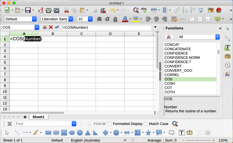
The Functions deck includes a brief description of each function and its arguments. Highlight the function and look at the bottom of the pane to see the description. If necessary, hover the mouse pointer over the division between the list and the description; when the pointer becomes a two-headed arrow, drag it upwards to increase the space for the description. Double-click on a function’s name to add it to the current cell, together with placeholders for each of the function’s arguments.
Using the Functions deck is almost as fast as manual entry, and has the advantage of not requiring that you memorize a formula that you want to use. In theory, it should also be less error-prone. In practice, though, some users may fumble when replacing the placeholders with values. Another feature is the ability to display the last formulas used.
The most commonly used input method is the Function Wizard (Figure 17). To open it, choose Insert > Function, or click the Function Wizard icon on the Formula Bar, or press Ctrl+F2. The Function Wizard provides the same help features as the Functions deck, but adds fields in which you can see the result of a completed function, as well as the result of any larger formula of which it is part.
Figure 17: Functions tab of Function Wizard
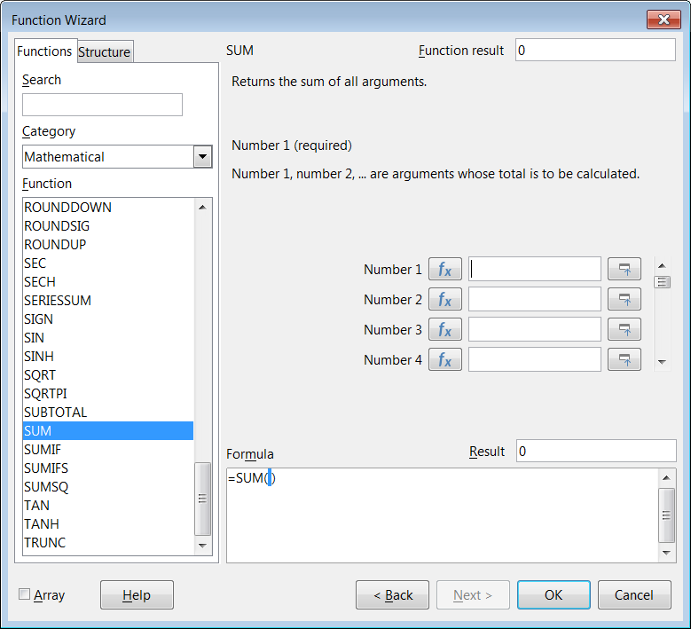
Select a category of functions to shorten the list, then scroll down through the named functions and select the required one by double-clicking on it. The available categories within the Function Wizard, and the number of functions available in each category, are given in Table 8. When you select a function its description appears on the right-hand side of the dialog. Optionally you can type the function name in the Search box and the search narrows on each character inserted (Figure 17).
Table 8: Function categories in the Function Wizard
|
Category |
Number of functions in category |
|
Add-in |
48 |
|
Array |
15 |
|
Database |
12 |
|
Date&Time |
36 |
|
Financial |
63 |
|
Information |
21 |
|
Logical |
11 |
|
Mathematical |
82 |
|
Spreadsheet |
22 |
|
Statistical |
151 |
|
Text |
47 |
The Function Wizard now displays an area to the right where you can enter data manually in text boxes or click the Shrink button to shrink the Function Wizard so you can select cells from the sheet.
Figure 18: Function Wizard after shrinking
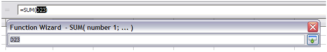
To select cells, either click directly on the cell or hold down the left mouse button and drag to select the required area.
When the area has been selected, click the Expand button to return to the wizard again.
If multiple arguments are needed click in the next text box and repeat the selection process for the next cell or range of cells. Repeat this process as often as required. The wizard will accept up to 255 ranges or arguments in the SUM function.
Click OK to accept the function, add it to the cell, and get the result.
Note
If you select a function by double-clicking it in the list, and then change your mind and select a different one by double-clicking again, then the second choice formula is added into the first choice formula in the Formula text box. You must clear the Formula text box and then double-click the function to add it to the box.
This additive facility allows you to create complex formulas by building them up in the Formula box.
You can also select the Structure tab to see a tree view of the parts of the formula. The main advantage over the Functions deck is that each argument is entered in its own field, making it easier to manage. The price of this reliability is slower input, but precision is generally more important than speed when creating a spreadsheet.
The structure view of the Function Wizard is important for debugging and fixing very long, nested, and complex formulas. In this view, the formula is parsed, and each formula component is calculated by a simpler function call or arithmetic operation and then combined following the rules of calculation. It is possible to visualize each parsed element of the formula and check if the intermediate results are correct, until the mistake is found.
Functions can be entered into the Input line. After you enter a function on the Input line, press the Enter key or click the Accept button on the Formula Bar to add the function to the cell and get its result.
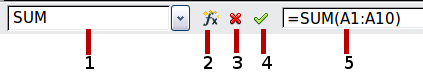
|
1 |
Name Box showing list of common functions |
||
|
2 |
Function Wizard |
4 |
Accept |
|
3 |
Cancel |
5 |
Input line |
Figure 19: The Formula Bar
If you see the formula in the cell instead of the result, then Formulas is selected in the Display section of the Tools > Options > LibreOffice Calc > View dialog. Deselect Formulas, and the result will display. However, you can still see the formula in the Input line.
Tip
The menu option View > Show Formula and the Windows / Linux shortcut Ctrl+` (grave accent) also toggle formulas on / off.
A formula in which the individual values in a cell range are evaluated is referred to as an array formula. The difference between an array formula and other formulas is that the array formula deals with several values simultaneously instead of just one.
Not only can an array formula process several values, but it can also return several values. The results of an array formula is also an array.
When Calc updates the formulas, each affected cell is read and its formula is recalculated. If you have a thousand cells in a column with the same formula (the formula expression only changes the data to compute), you end with one thousand identical formulas to interpret and execute.
Array formulas will evaluate the formula once and execute calculations as many time as the size of the array, thus saving the time used to interpret each cell formula. And because Calc stores only one formula for the entire array of data cells, it also save space in the spreadsheet file.
Figure 20: Source array in yellow and resulting array in green. The array formula is shown in the Formula Bar
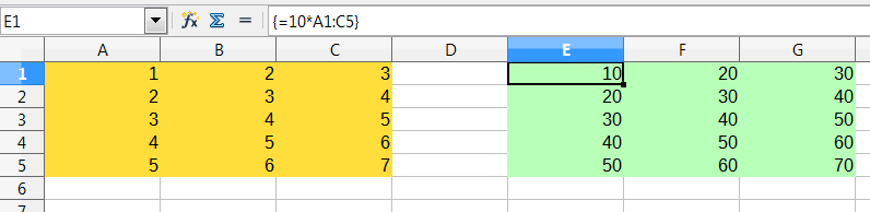
To multiply the values in the individual cells by 10 in the above array (Figure 20), you do not need to apply a formula to each individual cell or value. Instead you just need to use a single array formula. Select a range of 3 x 5 cells on another part of the spreadsheet, enter the formula =10*A1:C5 and confirm this entry using the key combination Ctrl+Shift+Enter. The result is a 3 x 5 array in which the individual values in the cell range (A1:C5) are multiplied by a factor of 10.
In addition to multiplication, you can also use other operators on the reference range (an array). With Calc, you can add (+), subtract (-), multiply (*), divide (/), use exponents (^), concatenation (&) and comparisons (=, <>, <, >, <=, >=). The operators can be used on each individual value in the cell range and return the result as an array if the array formula was entered.
Comparison operators in an array formula treat empty cells in the same way as in a normal formula, that is, either as zero or as an empty string. For example, if cells A1 and A2 are empty the array formulas {=A1:A2=""} and {=A1:A2=0} will both return a 1 column 2 row array of cells containing TRUE.
Use array formulas if you have to repeat calculations using different values. If you decide to change the calculation method later, you only have to update the array formula. To add an array formula, select the entire array range and then make the required change to the array formula.
Arrays are an essential tool for carrying out complex calculations, because you can have several cell ranges included in your calculations. Calc has different math functions for arrays, such as the MMULT function for multiplying two arrays.
If you create an array formula using the Function Wizard, you must mark the Array check box each time so that the results are returned in an array (Figure 17). Otherwise, only the value in the upper-left cell of the array being calculated is returned.
An array formula can also be entered directly into a cell. The result will automatically create an array of cells.
Note
Array formulas appear in braces (curly brackets) in Calc. You cannot create array formulas by manually entering the braces.
Note
The cells in a results array are automatically protected against changes. However, you can edit or copy the array formula by selecting the entire array cell range.
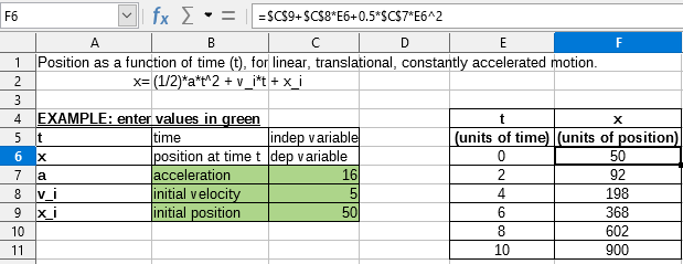
Formulas that do more than a simple calculation or summation of rows or columns of values usually take a number of arguments. For example, consider the following equation:
|
|
This equation models the position of an object undergoing linear, translational motion, with constant acceleration. The position (x) depends on time (t), and the equation also contains constant values for initial position (xi), initial velocity (vi), and acceleration (a).
For ease of presentation, it is good practice to set up a spreadsheet in a manner similar to that shown in Figure 21. In this example, the individual variables are input into cells on the sheet and no editing of the formula is required.
You can take several broad approaches when creating a formula. In deciding which approach to take, consider how many other people will need to use the sheets, the life of the sheets, and the variations that could be encountered in use of the formula.
If people other than yourself will use the spreadsheet, make sure that it is easy to see what input is required and where. Explanation of the purpose of the spreadsheet, basis of calculation, input required and output generated are often placed on the first sheet.
Figure 21: Setting up a formula with arguments
A spreadsheet that you build today, with many complicated formulas, may not be quite so obvious in its function and operation in 6 or 12 months. Use comments and notes liberally to document your work.
You might be aware that you cannot use negative values or zero values for a particular argument, but if someone else inputs such a value, will your formula be robust or simply return a standard (and often not too helpful) error message? It is a good idea to trap errors using some form of logic statements or with conditional formatting.
The most basic strategy is to view whatever formulas are needed as simple and with a limited useful life. The strategy is then to place a unique formula in each appropriate cell. This can be recommended only for very simple or “throw away” (single use) spreadsheets.
The second strategy is similar to the first, but instead you break down longer formulas into smaller parts and then combine the parts into the whole. Many examples of this type exist in complex scientific and engineering calculations where interim results are used in a number of places in the sheet. The result of calculating the flow velocity of water in a pipe may be used in estimating losses due to friction, whether the pipe is flowing full or partially empty, and in optimizing the diameter for the given flow regime.
In all cases you should adopt the basic principles of formula creation described previously.
Spreadsheets are often used to process raw data and produce meaningful summaries, consolidation and display of information for the decision maker, or to be used as the source for reports. The raw data can be produced by physical measurements, business transactions, or various other means. Sheets with thousands or even hundreds of thousands of rows and several columns are frequently found in finance departments or laboratories. Computations carried out on these raw data sets can be time consuming and last for minutes, hours and perhaps, days.
A common mistake is to insert formulas for each cell and perform thousands of formula interpretations and calculations. Here are some recommendation for speeding up calculations.
Array formulas have one formula applied to the mass of data. Computation saving can be significant for large data sets.
Consolidation functions perform calculations on data sets. SUM, SUMIF, SUMIFS, SUMPRODUCT are examples of consolidation functions. For example if you have a very long bill of materials (BOM), where quantity must be multiplied by unit price and then totaled to produce a cost figure, then instead of applying a formula on each entry of the BOM and then summing, you can use the formula SUMPRODUCT(quantity, unitprice), where quantity and unitprice are named ranges representing the BOM. SUMPRODUCT multiplies each cell of the quantity data set by its corresponding cell of unitprice and sums all the products.
Similar situations happen when you must sum a subset of the original data set, where you must apply a test on each entry to allow it to be part of the sum. For example, when the value is strictly positive. Use SUMIF(data_to_test;”>0”;data_to_sum), where data_to_test is the data set where you test the positive values, data_to_sum is the column where the values are to sum depending on the test, and “>0” is the test itself.
Other consolidation functions are AVERAGEIF, COUNTIF, MINIFS, MAXIFS, and more.
Another strategy is to create your own functions and macros. This approach would be used where the result would greatly simplify the use of the spreadsheet by the end user and keep the formulas simple with a better chance of avoiding errors. This approach also can make the maintenance easier by having corrections or updates kept in one central location. The use of macros is described in Chapter 13, Macros, and is a specialized topic in itself. The danger of overusing macros and custom functions is that the principles upon which the spreadsheet is based become much more difficult to see by a user other than the original author (and sometimes even by the author!).
Many modern computers have multi-core processors and provide for multiple threads. A core is a physical hardware component within a CPU. Threads are virtual components that help to efficiently manage the workload and tasks of the CPU. A CPU can interact with more than one thread at a time and multi-threading makes CPUs more efficient, to give better overall performance.
Calc supports multi-threading to help your spreadsheets take advantage of whatever parallel processing is available within your computer. This facility is controlled by the Enable multi-threaded calculation option in the CPU Threading Settings section of the Tools > Options > LibreOffice Calc > Calculate dialog. The initial default is for this option to be enabled, and disabling it is not recommended. This is the only control in the Calc user interface that relates to multi-threading; once initiated, the processing operates automatically.
If multi-threading is enabled, Calc automatically identifies where your spreadsheet could benefit from multi-threading and processes it accordingly. Threads are generally used for formula groups, where enough adjacent cells in a column use the same formula but get different results because of relative cell addressing. One implication of this approach is that the optimization is column-based and so a row-based layout could be less efficient.
There are other ways to control Calc’s multi-threading capability, such as adjusting the MAX_CONCURRENCY LibreOffice specific environment variable. However, these methods are beyond the scope of this document.
It is common to find situations where errors are displayed. Even with all the tools available in Calc to help you to enter formulas, making mistakes is easy. Many people find inputting numbers difficult and many may make a mistake about the kind of entry that a function’s argument needs. In addition to correcting errors, you may want to find the cells used in a formula to change their values or to check the answer.
Calc provides three tools for investigating formulas and the cells that they reference: error messages, color coding for input, and the Detective.
The most basic tool is error messages. Error messages display in a formula’s cell, on the Status Bar, or in the Function Wizard instead of the result.
An error message for a formula is usually a three-digit number from 501 to 540, or sometimes an unhelpful piece of text such as #NAME?, #REF!, or #VALUE!. The error message appears in the cell, and a brief explanation of the error is shown on the right side of the Status bar.
Most error messages indicate a problem with how the formula was input, although several indicate that you have run up against a limitation of either Calc or its current settings.
Error messages are not user-friendly, and may intimidate new users. However, they are valuable clues to correcting mistakes. You can find detailed explanations of them in Appendix B, Error Codes, and in the Help, by searching for “error codes” in Calc. A few of the most common are shown in Table 9.
Table 9: Common error messages
|
Code |
Meaning |
|
#NAME? |
Instead of displaying Err:525. No valid reference exists for the argument. |
|
#REF! |
Instead of displaying Err:524. The column, row, or sheet for the referenced cell is missing. |
|
#VALUE! |
Instead of displaying Err:519. The value for one of the arguments is not the type that the argument requires. The value may be entered incorrectly; for example, double-quotation marks may be missing around the value. At other times, a cell or range used may have the wrong format, such as text instead of numbers. |
|
#DIV/0! |
Instead of displaying Err:532. Division by zero. |
|
#NUM! |
Instead of displaying Err:503. A calculation results in an overflow of the defined value range. |
|
509 |
An operator such as an equals sign is missing from the formula. |
|
510 |
A variable is missing from the formula. |
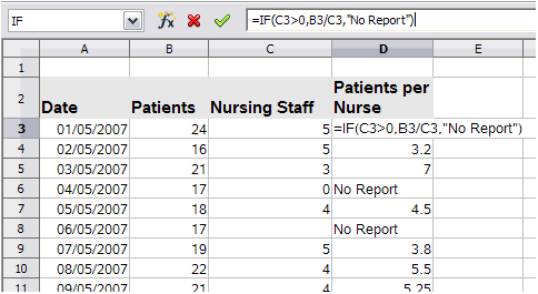
This error is the result of dividing a number by either the number zero (0) or a blank cell. There is an easy way to avoid this type of problem. When you have a zero or blank cell displayed, use a conditional function. Figure 22 depicts division of column B by column C yielding 2 errors arising from a zero and a blank cell showing in column C.
It is very common to find an error such as this arising from a situation where data was not reported or reported incorrectly. When such an occurrence is possible, an IF function can be used to display the data correctly. The formula =IF(C3>0, B3/C3, “No Report”) can be entered. The formula is then copied over the remainder of column D. The meaning of this formula roughly would be: “If C3 is greater than 0, then compute B3 divided by C3, otherwise enter ‘No Report’”. An example is shown in Figure 23.
It is also possible for the last parameter to use double quotes for a blank (no value) to be entered, or a different formula with a standardized number being substituted for the lower number.
Figure 22: Examples of #DIV/0!, division by zero error
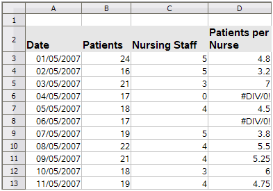
Figure 23: Division by zero solution
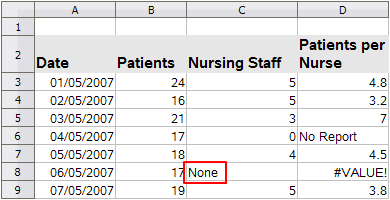
The #VALUE! error is also very common.
A common occurrence of this error arises when a cell contains an incorrect value type. In the example of Figure 24, text “None” has been entered in C8, where our formula in column D is expecting a number.
Figure 24: Incorrect entry causing #VALUE! error
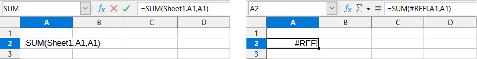
The #REF! error is caused by a missing reference. In the example shown in Figure 25, the formula references a sheet that has been deleted.
Figure 25: Deleted sheet causing #REF! error
Another useful tool when reviewing a formula is the color coding for input. When you select a formula that has already been entered, the cells or ranges used for each argument in the formula are outlined in color.
Figure 26: Color coding for input
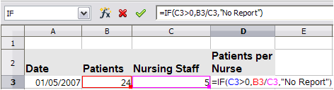
Calc uses eight colors for outlining referenced cells, starting with blue for the first cell, and continuing with red, magenta, green, dark blue, brown, purple, and yellow before cycling through the sequence again.
There are situations where the display of cell contents is the same when the data type is different. For example text contents and numeric contents can look the same but can produce a mistake if both are used in some calculations. To illustrate, the string “10.35” right-aligned in a cell can be confused with the value 10.35. When the cell is used in a formula the string may take the value of zero and an error may be produced.
If you enable value highlighting (View > Value Highlighting or Ctrl+F8), Calc distinguishes the text and numeric data types by assigning different colors to the content’s characters. By default, the text contents are in black characters and the numeric contents are in blue. See Chapter 2, Entering and Editing Data, for more information on value highlighting.
In a long or complicated spreadsheet, color coding becomes less useful. In these cases, consider using the submenu under Tools > Detective. The Detective is a tool for checking which cells are used as arguments by a formula (precedents) and which other formulas it is nested in (dependents), and tracking errors. It can also be used for tracing errors, marking invalid data (that is, information in cells that is not in the proper format for a function’s argument), or even for removing precedents and dependents.
To use the Detective, select a cell with a formula, then select the required option in the Tools > Detective menu. On the spreadsheet, you will see lines ending in dots to indicate precedents, and lines ending in arrows for dependents. The lines show the flow of information.
Use the Detective to assist in following the precedents referred to in a formula in a cell. By tracing these precedents, you frequently can find the source of the errors. Place the cursor in the cell in question and then choose Tools > Detective > Trace Precedents on the Menu bar or press Shift+F9. Figure 27 shows a simple example of tracing precedents for cell B4.
This allows us to check the source cells (which may be a range) for any errors which have caused us to query the calculation result. If a source is a range, then that range is highlighted in blue.
Figure 27: Tracing precedents using the Detective
In other instances we may have to trace an error. For this we use the Trace Error function, found under Tools > Detective > Trace Error, to find the cells that caused the error.
For more information search for “Detective” in the Help system’s index.
For novices, functions are one of the most intimidating features of LibreOffice Calc. New users quickly learn that functions are an important feature of spreadsheets, but there are hundreds, and many require input that assumes specialized knowledge. Fortunately, Calc includes many functions that anyone can use.
The most basic functions create formulas for basic arithmetic or for evaluating numbers in a range of cells.
The simple arithmetic functions are addition, subtraction, multiplication, and division. Except for subtraction, each of these operations has its own function:
SUM for addition
PRODUCT for multiplication
QUOTIENT for division
SUM, PRODUCT, and QUOTIENT are useful for entering ranges of cells in the same way as any other function, with arguments in brackets after the function name.
However, for basic equations, many users prefer the time-honored computer symbols for these operations, using the plus sign (+) for addition, the hyphen (–) for subtraction, the asterisk (*) for multiplication and the forward slash (/) for division. These symbols are quick to enter without requiring your hands to stray from the keyboard.
A similar choice is also available if you want to raise a number by the power of another. Instead of entering =POWER(A1,2), you can enter =A1^2.
Moreover, they have the advantage that you enter formulas with them in an order that more closely approximates human readable format than the spreadsheet-readable format used by the equivalent function. For instance, instead of entering =SUM(A1:A2), or possibly =SUM(A1,A2), you enter =A1+A2. This almost-human readable format is especially useful for compound operations, where writing =A1*(A2+A3) is briefer and easier to read than =PRODUCT(A1,SUM(A2:A3)).
The main disadvantage of using arithmetical operators is that you cannot directly use a range of cells. In other words, to enter the equivalent of =SUM(A1:A3), you would need to type =A1+A2+A3.
Otherwise, whether you use a function or an operator is largely up to you—except, of course, when you are subtracting. However, if you use spreadsheets regularly in a group setting such as a class or an office, you might want to standardize on an entry format so that everyone who handles a spreadsheet becomes accustomed to a standard input.
Another common use for spreadsheet functions is to pull useful information out of a list, such as a series of test scores in a class, or a summary of earnings per quarter for a company.
You can, of course, scan a list of figures if you want basic information such as the highest or lowest entry or the average. The only trouble is, the longer the list, the more time you waste and the more likely you are to miss what you are looking for. Instead, it is usually quicker and more efficient to enter a function. Such reasons explain the existence of a function like COUNT, which does no more than give the total number of entries in the designated cell range.
Similarly, to find the highest or lowest entry, you can use MIN or MAX. For each of these formulas, all arguments are either a range of cells, or a series of cells entered individually.
Each also has a related function, MINA or MAXA, which performs the same function, but also treats a cell formatted for text as having a value of 0. (The same treatment of text occurs in any variation of another function that adds an "A" to the end.) Either function gives the same result, and could be useful if you used a text notation to indicate, for example, if any students were absent when a test was written, and you wanted to check whether to schedule a makeup exam.
For more flexibility in similar operations, you could use LARGE or SMALL, both of which add a specialized argument of rank. If the rank is 1 used with LARGE, you get the same result as you would with MAX. However, if the rank is 2, then the result is the second largest result. Similarly, a rank of 2 used with SMALL gives you the second smallest number. Both LARGE and SMALL are handy as a permanent control, since, by changing the rank argument, you can quickly scan multiple results.
You would need to be an expert to want to find the Poisson distribution of a sample, or to find the skew or negative binomial of a distribution (and, if you are, you will find functions in Calc for such things). However, for the rest of us, there are simpler statistical functions that you can quickly learn to use.
In particular, if you need an average, you have a number of functions to choose from. You can find the arithmetical mean—that is, the result when you add all entries in a list then divide by the number of entries, by entering a range of numbers when using AVERAGE, or AVERAGEA to include text entries and to give them a value of zero.
In addition, you can get other information about the data set:
MEDIAN: Logically ranks the numbers (lowest to highest) to evaluate the median value. In a set containing an uneven number of values, the median will be the number in the middle of the ranked list. In a set containing an even number of values, the median will be the mean of the two values in the middle of the ranked list.
MODE: The most common entry in a list of numbers.
QUARTILE: The entry at a set position in the array of numbers. Besides the cell range, you enter the type of quartile: 0 for the lowest entry, 1 for the value of 25%, 2 for the value of 50%, 3 for 75%, and 4 for the highest entry. Note that the result for types 1 through 3 may not represent an actual item entered.
RANK: The position of a given entry in the entire list, measured either from top to bottom or bottom to top. You need to enter the cell address for the entry, the range of entries, and the type of rank (0 for the rank from the highest, or any other value for the rank from the bottom).
Some of these functions overlap; for example, MIN and MAX are both covered by QUARTILE. In other cases, a custom sort or filter might give much the same result. Which you use depends on your temperament and your needs. Some might prefer to use MIN and MAX because they are easy to remember, while others might prefer QUARTILE because it is more versatile.
In some cases, you may be able to get similar results to some of these functions by setting up a filter or a custom sort. However, in general, functions are more easily adjusted than filters or sorts, and provide a wide range of possibilities.
At times, you may just want to enter one or more formulas temporarily in a convenient blank cell, and delete it once you have finished. However, if you find yourself using the same functions constantly, you should consider creating a template and including space for all the functions you use, with the cell to their left used as a label for them. Once you have created the template, you can easily update each formula as entries change, either automatically and on-the-fly or pressing the F9 key to update all selected cells.
No matter how you use these functions, you will probably find them simple to use and adaptable for many purposes. By the time you have mastered this handful, you will be ready to try more complex functions.
For statistical and mathematical purposes, Calc includes a variety of ways to round off numbers. If you are a programmer, you may also be familiar with some of these methods. However, you do not need to be a specialist to find some of these methods useful. You may want to round off for billing purposes, or because decimal places do not translate well into the physical world—for instance, if the parts you need come in packages of 100, then the fact you only need 66 is irrelevant to you; you need to round up for ordering. By learning the options for rounding up or down, you can make your spreadsheets more immediately useful.
When you use a rounding function, you have two choices about how to set up your formulas. If you choose, you can nest a calculation within one of the rounding functions. For instance, the formula =ROUND((SUM(A1,A2)) adds the figures in cells A1 and A2, then rounds them off to the nearest whole number. However, even though you do not need to work with exact figures every day, you may still want to refer to them occasionally. If that is the case, then you are probably better off separating the two functions, placing =SUM(A1,A2) in cell A3, and =ROUND(A3) in A4, and clearly labeling each function.
For details on rounding methods, see the Help.
The Open Document Format for Office Applications (OpenDocument) Version 1.2 includes the following definition: “Functions that are always recalculated whenever a recalculation occurs are termed volatile functions.”
To understand some of the behaviors of a volatile function within Calc, consider a simple example in which you have created an empty spreadsheet and entered the formula =RAND() into cell A1 (RAND is one of Calc’s volatile functions). Calc displays a random number between 0 and 1 in cell A1. If you then enter any value into a different cell (say cell B2 for the purpose of this discussion) and press Enter, you will notice that the value displayed in A1 is updated to show a different random number. Calc recalculates the random number in A1, despite the user not changing the formula in A1 and despite the updated B2 having no link to A1. In summary, the RAND function will generate a new value when any cell is updated by selecting Data > Calculate > Recalculate or pressing F9, or on any input event.
An understanding of volatile functions is important especially if you create a large spreadsheet, where frequent recalculations may adversely affect performance. Make sure that you design your spreadsheet to use volatile functions appropriately.
The following Calc functions are volatile:
FORMULA
INDIRECT
INFO
NOW
OFFSET
RAND
RANDBETWEEN
TODAY
For the RAND and RANDBETWEEN functions, Calc provides non-volatile equivalents – RAND.NV and RANDBETWEEN.NV. These may be useful when you do not require the function values to update so frequently. A non-volatile function is not recalculated at new input events and does not recalculate when selecting Data > Calculate > Recalculate or pressing F9, except when the cell containing the function is selected. Non-volatile functions are recalculated when opening the file.
Calc supports the use of regular expressions or wildcards in the arguments of many of its functions.
Regular expressions offer the most powerful method of searching for text strings. For more information about regular expressions, including examples, see the section entitled “Regular expressions” in Chapter 1, Introduction.
If interoperability with Microsoft Excel is important for your spreadsheet, then you may not be able to fully utilize Calc’s regular expression facilities because Excel does not provide equivalent facilities. Hence, when you export a Calc spreadsheet to Excel format, information relating to regular expressions will not be usable within Excel. In this case you can use the less powerful wildcards facility provided by Calc because spreadsheets that utilize wildcards can be exported to Excel format without loss of data. A wildcard is a special character that represents one or more unspecified characters. Wildcards make text searches more powerful, but often less specific. The wildcards available are ? (question mark), * (asterisk), and ~ (tilde). The usage of these wildcards is the same as that for the Find and Replace dialog, described in Section 2, Entering, Editing, and Formatting Data.
The following Calc functions allow the use of wildcards or regular expressions:
Database functions (DAVERAGE, DCOUNT, DCOUNTA, DGET, DMAX, DMIN, DPRODUCT, DSTDEV, DSTDEVP, DSUM, DVAR, DVARP)
AVERAGEIF, AVERAGEIFS, COUNTIF, COUNTIFS, MAXIFS, MINIFS, SUMIF, SUMIFS
HLOOKUP, LOOKUP, VLOOKUP
MATCH
REGEX (not applicable for wildcards)
SEARCH
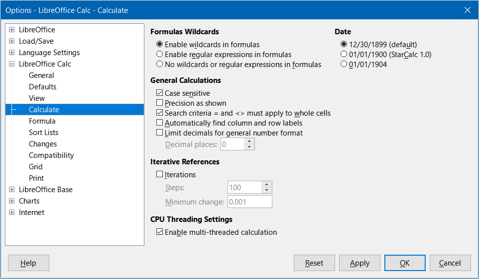
Configuration options are available in the Formulas wildcards section on the Tools > Options > LibreOffice Calc > Calculate dialog (Figure 28) to control the use of wildcards and regular expressions with Calc’s functions. The three mutually exclusive, self-explanatory options are:
Enable wildcards in formulas. This is the initial default when Calc is installed.
Enable regular expressions in formulas.
No wildcards or regular expressions in formulas.
A further related option in the General Calculations area of the same dialog, Search criteria = and <> must apply to whole cells, controls whether search criteria must match the whole cell exactly.
By default, regular expression searches within Calc functions are case insensitive, irrespective of the setting of the Case sensitive checkbox. However, for some functions regular expressions can include a flag option “(?-i)” to switch to a case sensitive match. Functions that support this facility are: AVERAGEIF, AVERAGEIFS, COUNTIF, COUNTIFS, HLOOKUP, LOOKUP, MATCH, SEARCH, SUMIF, SUMIFS, and VLOOKUP.
Figure 28: Tools > Options > LibreOffice Calc > Calculate dialog
Tip
When both the Search criteria = and <> must apply to whole cells and Enable wildcards in formulas options are selected, Calc behaves exactly as Microsoft Excel when searching cells in the database functions.
To illustrate some of the features of regular expressions, consider the simple spreadsheet shown in Figure 29 and assume that Enable regular expressions in formulas is selected.
Figure 29: Using the COUNTIF function

1) With the formula =COUNTIF(A1:A6,”r.d”) entered in cell A7 and Search criteria = and <> must apply to whole cells deselected, the value 5 is displayed in cell A7, as shown in Figure 29. The formula counts cells in the range A1:A6 which contain “Fred”, “red”, “ROD”, “bride”, and “Ridge”.
2) With the formula =COUNTIF(A1:A6,”(?-i)r.d”) entered in cell A7 and Search criteria = and <> must apply to whole cells deselected, the value 3 is displayed in cell A7. The formula counts cells in the range A1:A6 which contain “Fred”, “red”, and “bride”. This regular expression utilizes the “(?-i)” flag option to perform a case sensitive search.
3) With the formula =COUNTIF(A1:A6,”r.d”) entered in cell A7 and Search criteria = and <> must apply to whole cells selected, the value 2 is shown in cell A7. The formula counts cells in the range A1:A6 which contain “red” and “ROD”.
4) With the formula =COUNTIF(A1:A6,”(?-i)r.d”) entered in cell A7 and Search criteria = and <> must apply to whole cells selected, the value 1 is shown in cell A7. The formula counts cells in the range A1:A6 which contain “red”. This regular expression utilizes the “(?‑i)” flag option to perform a case sensitive search.
5) With the formula =COUNTIF(A1:A6,".*r.d.*") entered in cell A7 and Search criteria = and <> must apply to whole cells selected, the value 5 is again shown in cell A7. Contrast this with example ) above – the regular expression in the current example allows for 0 or more characters both before the “r” and after the “d”.
Regular expressions will not work in simple comparisons. For example: A1=“r.d” will always return FALSE if A1 contains red, even if regular expressions are enabled. It will only return TRUE if A1 contains r.d (r then a dot then d). If you wish to test using regular expressions, try the COUNTIF function: COUNTIF(A1, “r.d”) will return 1 or 0, interpreted as TRUE or FALSE in formulas like =IF(COUNTIF(A1, “r.d”), “hooray”, “boo”).
Activating the Enable regular expressions in formulas option means all the above functions will require any regular expression special characters (such as parentheses) used in strings within formulas to be preceded by a backslash, despite not being part of a regular expression. These backslashes will need to be removed if the setting is later deactivated.
As is common with other spreadsheet programs, Calc can be enhanced by user-defined functions or add-ins. Setting up user-defined functions can be done either by using macros or by writing separate add-ins or extensions.
The basics of writing and running macros is covered in Chapter 13, Macros. Macros can be linked to menus or toolbars for ease of operation or stored in template modules to make the functions available in other documents. Calc macros can be written in Basic, BeanShell, JavaScript, or Python.
Calc Add-ins are specialized office extensions which can extend the functionality of LibreOffice with new built-in Calc functions. A number of extensions for Calc have been written; these can be found on the extensions site at https://extensions.libreoffice.org/. Refer to Chapter 15, Setting up and Customizing, for more details.