
Calc Guide 7.5
Chapter 4
Formatting Data
Make your data shine
This document is Copyright © 2023 by the LibreOffice Documentation Team. Contributors are listed below. This document maybe distributed and/or modified under the terms of either the GNU General Public License (https://www.gnu.org/licenses/gpl.html), version 3 or later, or the Creative Commons Attribution License (https://creativecommons.org/licenses/by/4.0/), version 4.0 or later. All trademarks within this guide belong to their legitimate owners.
To this edition
Olivier Hallot
To previous editions
Skip Masonsmith
Roman Kuznetsov
flywire
Steve Fanning
Jenna Sargent
Pulkit Krishna
Jean Hollis Weber
Dan Lewis
Peter Schofield
Jochen Schiffers
Robert Großkopf
Jost Lange
Martin Fox
Hazel Russman
Steve Schwettman
Alain Romedenne
Andrew Pitonyak
Jean-Pierre Ledure
Drew Jensen
Randolph Gamo
Please direct any comments or suggestions about this document to the Documentation Team’s forum at https://community.documentfoundation.org/c/documentation/loguides/ (registration is required) or send an email to: loguides@community.documentfoundation.org.
Note
Everything sent to a forum, including email addresses and any other personal information that is written in the message, is publicly archived and cannot be deleted. E-mails sent to the forum are moderated.
Published February 2023. Based on LibreOffice 7.5 Community.
Other versions of LibreOffice may differ in appearance and functionality.
Some keystrokes and menu items are different on macOS from those used in Windows and Linux. The table below gives some common substitutions used in this document. For a detailed list, see LibreOffice Help.
|
Windows or Linux |
macOS equivalent |
Effect |
|
Tools > Options |
LibreOffice > Preferences |
Access setup options |
|
Right-click |
Control+click or right-click depending on computer setup |
Open a context menu |
|
Ctrl or Control |
⌘ and/or Cmd or Command, depending on keyboard |
|
|
Alt |
⌥ and/or Alt or Option depending on keyboard |
Used with other keys |
|
F11 |
⌘+T |
Open Styles deck in Sidebar |
Cell formatting is an important feature of any modern spreadsheet software including Calc. Calc formatting resources use an extensive set of attributes to enhance the visual display of relevant information of your spreadsheet. Manual and style formatting as well as conditional formatting are addressed in this chapter.
Note
All the settings discussed in this section can also be set as a part of the cell style. See Chapter 5, Using Styles and Templates, for more information.
You can format the data in Calc in several ways, either defined as part of a cell style so that it is automatically applied, or applied manually to the cell. For more control and extra options, select a cell or cell range and use the Format Cells dialog. All of the format options are discussed below.
Multiple lines of text can be entered into a single cell using automatic wrapping or manual line breaks. Each method is useful for different situations.
To automatically wrap multiple lines of text in a cell, use one of the following methods:
Method 1
1) Select a cell or cell range.
2) Go to Format > Cells on the Menu bar, or right-click and select Format Cells in the context menu, or press Ctrl+1, to open the Format Cells dialog.
3) Click on the Alignment tab (Figure 1).
4) Under Properties, select Wrap text automatically and click OK.
Method 2
1) Select the cell.
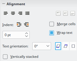
2) On the Properties deck of the Sidebar, open the Alignment panel (Figure 2).
3) Select the Wrap text option to apply the formatting immediately.
Method 3
1) Select the cell.
2) Click on the toolbar Wrap Text tool.
Figure 1: Format Cells dialog – Alignment tab
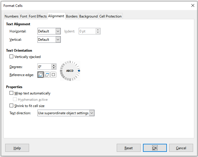
Figure 2: Wrap text formatting
To insert a manual line break while typing in a cell, press Ctrl+Enter. When editing text, double-click the cell, then reposition the cursor to where you want the line break. In the Input line of the Formula bar, you can also press Shift+Enter.
When a manual line break is entered, the cell row height changes but the cell width may not change and the text may still overlap the end of the cell. You have to change the cell width manually or reposition the line break.
The font size of the data in a cell can automatically adjust to fit inside cell borders:
1) Select a cell or cell range.
2) Go to Format > Cells on the Menu bar, or right-click and select Format Cells in the context menu, or press Ctrl+1, to open the Format Cells dialog.
3) Click on the Alignment tab (Figure 1).
4) Under Properties, select Shrink to fit cell size and click OK.
Several number formats can be applied to cells by using icons on the Formatting toolbar (highlighted in Figure 3). Select the cell, then click the relevant icon to change the number format.
For more control or to select other number formats, use the Numbers tab of the Format Cells dialog (Figure 1 above):
Apply any of the data types in the Category list to the data.
Select one of the predefined formats in the Format list.
Control the number of decimal places and leading zeroes in Options.
Enter a custom format code. This is a very powerful facility that is detailed in the Number Format Codes page of the Help.
The Language setting controls the local settings for the different formats such as the date format and currency symbol.
Figure 3: Number icons on Formatting toolbar

To select a font and format it for use in a cell:
1) Select a cell or cell range.
2) Click the down arrow on the right of the Font Name box on the Formatting toolbar (highlighted in Figure 4) and select a font in the drop-down list. The font can also be changed using the Font tab on the Format Cells dialog.
3) Click on the down arrow on the right of the Font Size box on the Formatting toolbar and select a font size from the drop-down list. The font size can also be changed using the Font tab on the Format Cells dialog.
4) To change the character format, click on the Bold, Italic, or Underline icons on the Formatting toolbar.
5) To change the paragraph alignment, click on one of the alignment icons (Align Left, Align Center and Align Right). The Format > Align menu also provides these options in addition to the Justified alignment.
Figure 4: Font Name and Size on Formatting toolbar

Note
To specify the language used in the cell, open the Font tab on the Format Cells dialog. Changing language in a cell allows different languages to exist within the same document. For more changes to font characteristics, see “Font effects” below.
Tip
To choose whether to show the font names in their font or in plain text, go to Tools > Options > LibreOffice > View and select or deselect the Show preview of fonts option in the Font Lists section. For more information, see Chapter 15, Setting up and Customizing.
1) Select a cell or cell range.
2) Right-click and select Format Cells in the context menu, or go to Format > Cells on the Menu bar, or press Ctrl+1, to open the Format Cells dialog.
3) Click on the Font Effects tab (Figure 5).
Figure 5: Format Cells dialog – Font Effects tab
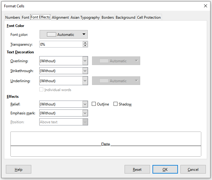
4) Select the font effect you want to use from the options available. The options available are described in Chapter 5, Using Styles and Templates.
5) Click OK to apply the font effects and close the dialog.
Any font effect changes are applied to the current selection, or to the entire word that contains the cursor, or to any new text that you type.
To change the text direction within a cell, use the Alignment tab on the Format Cells dialog (Figure 1 above):
1) On the Alignment tab of the Format Cells dialog, select the Reference edge from which to rotate the text as follows:
Text Extension From Lower Cell Border – writes the rotated text from the bottom cell edge outwards.
Text Extension From Upper Cell Border – writes the rotated text from the top cell edge outwards.
Text Extension Inside Cell – writes the rotated text only within the cell.
2) Click on the small indicator at the edge of the text orientation dial and rotate it until you reach the required degrees.
3) Alternatively, enter the number of degrees to rotate the text in the Degrees box.
4) Select Vertically stacked to make the text appear vertically in the cell.
An Asian layout mode checkbox is available on the Alignment tab of the Format Cells dialog when Asian language support is enabled and the text direction is set to vertical. This option aligns Asian characters one below the other in the selected cell(s). If the cell contains more than one line of text, the lines are converted to text columns that are arranged from right to left. Western characters in the converted text are rotated 90 degrees to the right. Asian characters are not rotated.
The tools on the Formatting toolbar can be used as follows after the cell has been selected:
To change the text direction from horizontal (default direction) to vertical, click on the Text direction from top to bottom icon.
To change text direction from vertical to horizontal (default), click on the Text direction from left to right icon.
To change text direction from left to right, which is the default direction for Western fonts, to a right to left direction used in some fonts, for example Arabic, then click on the Right-To-Left icon. This only works if a font has been used that requires a right to left direction.
To change text direction back to the default left to right direction used for Western fonts, click on the Left-To-Right icon.
Note
The text direction icons can only be made available if the Asian and Complex text layout options are checked under Tools > Options > Language Settings > Languages > Default Language for Documents. If it is necessary to make the buttons visible, right-click on the toolbar and select Visible Buttons in the context menu, then click on the icon you require and it will be placed on the Formatting toolbar.
If Asian language support is enabled through Tools > Options > Language Settings > Languages > Default Languages for Documents > Asian, an Asian Typography tab is included on the Format Cells dialog (Figure 6). This tab enables setting of typographic options for cells in Asian language documents.
Figure 6: Format Cells dialog - Asian Typography tab
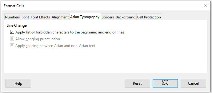
The following options are provided:
Apply list of forbidden characters to the beginning and end of lines – prevents the characters in the list of restricted characters from starting or ending a line. The characters are relocated to either the previous or the next line. To edit the list of restricted characters, go to Tools > Options > Language Settings > Asian Layout > First and Last Characters.
Allow hanging punctuation – prevents commas and periods from breaking the line. Instead, these characters are added to the end of the line, even in the page margin.
Apply spacing between Asian and non-Asian text – inserts a space between ideographic and alphabetic text.
To format the borders of a cell or a group of selected cells, you can use the border icons on the Formatting toolbar to apply the default styles to borders, or the Format Cells dialog for greater control. See Chapter 5, Using Styles and Templates, for more information on the options:
Note
Cell border properties apply only to the selected cells and can only be changed if you are editing those cells. For example, if cell C3 has a top border, that border can only be removed by selecting C3. It cannot be removed in C2, even though it appears to be the bottom border for cell C2.
1) Select a cell or a range of cells.
2) Go to Format > Cells on the Menu bar, or right-click and select Format Cells in the context menu, or press Ctrl+1, to open the Format Cells dialog.
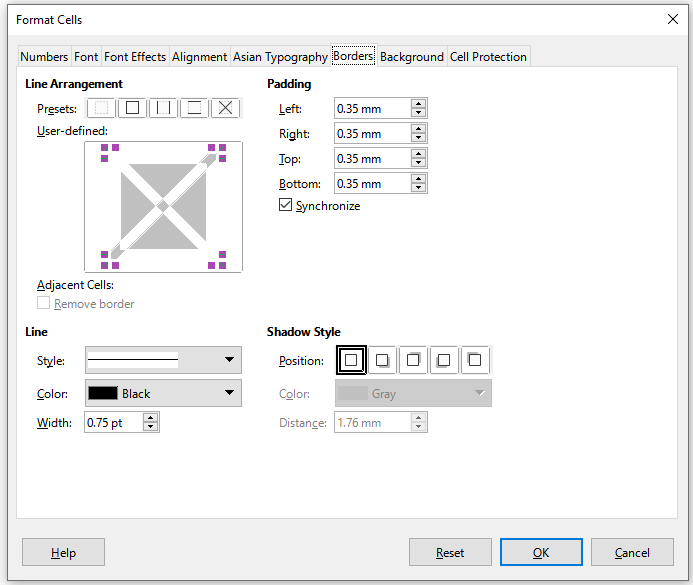
3) On the Borders tab (Figure 7), select the options required.
4) Click OK to close the dialog and save the changes.
Alternatively, use the icons on the Formatting toolbar to apply default styles to borders:
1) Click the Borders icon and select one of the options displayed in the Borders palette.
2) Click the Border Style icon and select one of the line styles from the Border Style palette.
3) Click the Border Color icon to apply the most recently selected color. Click the down arrow to the right of the Border Color icon to select another color from the Border Color palette.
Note
When entering borders with the border icons on the Formatting toolbar, you have two choices: click the required icon to add a border to the present borders or Shift-click to add a border and remove the present borders.
Figure 7: Format Cells dialog – Borders tab
To format the background color for a cell or a group of cells (see Chapter 5, Using Styles and Templates, for more information):
1) Select a cell or a range of cells.
2) Go to Format > Cells on the Menu bar, or right-click and select Format Cells in the context menu, or press Ctrl+1, to open the Format Cells dialog.
3) On the Background tab, click the Color button and select a color from the color palette.
4) Click OK to save the changes and close the dialog.
Alternatively, click on the Background Color icon on the Formatting toolbar to apply the most recently selected color. Click the down arrow to the right of the Background Color icon to select a different color from the Background Color palette.
You can use AutoFormat to format a group of cells:
1) Select the cells in at least three columns and rows, including column and row headers, that you want to format.
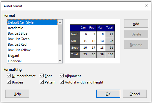
2) Go to Format > AutoFormat Styles on the Menu bar to open the AutoFormat dialog (Figure 8).
3) Select the type of format and format color in the list.
4) Select the formatting properties to be included in the AutoFormat function.
5) Click OK to apply the changes and close the dialog.
Figure 8: AutoFormat dialog
You can define a new AutoFormat so that it becomes available for use in all spreadsheets:
1) Format the data type, font, font size, cell borders, cell background, and so on for a group of cells.
2) Select a cell range of at least 4x4 cells.
3) Go to Format > AutoFormat Styles to open the AutoFormat dialog. The Add button is now active (if a range smaller than 4x4 cells is selected, the Add button will be unavailable).
4) Click Add.
5) In the Name box of the Add AutoFormat dialog that opens, type a meaningful name for the new format and click OK.
6) The new AutoFormat is now available in the Format list on the AutoFormat dialog. Click OK to close the AutoFormat dialog.
Note
Autoformatting does not use cell styles. It applies direct formatting to the selected range. The new Autoformat is stored in the user profile and is not part of the spreadsheet document. This means that you can reuse the new AutoFormat in another spreadsheet document using your profile but under a different profile or different user, the new AutoFormat will not be listed. See Chapter 5, Using Styles and Templates.
Sometimes your spreadsheet can contain data of different types in the same column, row or range. For example, a column with dates can have a string (text) written in the same format as the default date format for the column. Because strings and numbers are treated differently in some important functions like AVERAGE, the spreadsheet can display wrong results if your data has mixed types.
Value highlighting displays cell contents in different colors depending on the type of content. An example of value highlighting is shown in Figure 9:
Text is shown in black.
Formulas are shown in green.
Numbers (including date and time) are shown in blue.
Figure 9: Example of value highlighting
The value highlighting colors override any colors used in formatting. This color change applies only to the colors seen on a display. When a spreadsheet is printed, the original colors used for formatting are printed.
Go to View > Value Highlighting on the Menu bar, or use the keyboard shortcut Ctrl+F8, to turn the function on or off. When value highlighting is switched off, the original formatting colors are used for display.
You can make value highlighting the default when opening a spreadsheet in Calc, by selecting Tools > Options > LibreOffice Calc > View > Display > Value highlighting. This default mode for value highlighting may not be what you want if you are going to format the cells for printing.
You can set up cell formats to change depending on conditions that you specify. Conditional formatting is used to highlight data that is outside the specifications that you have set. It is recommended not to overuse conditional formatting as this could reduce the impact of data that falls outside those specifications.
Note
Conditional formatting depends upon the use of styles and the AutoCalculate feature must be enabled. If you are not familiar with styles, see Chapter 5, Using Styles and Templates, for more information.
1) Ensure that AutoCalculate is enabled: Data > Calculate > AutoCalculate.
2) Select the cells where you want to apply conditional formatting.
3) Go to Format > Conditional > Condition (Figure 14), Color Scale (Figure 19), Data Bar (Figure 20), Icon Set (Figure 22), or Date (Figure 18), on the Menu bar to open the Conditional Formatting dialog. Any conditions already defined are displayed.
4) Click Add to create and define a new condition. Repeat this step as necessary.
5) Select a style from the styles already defined in the Apply Style drop-down list. Repeat this step as necessary.
6) Alternatively, select New Style to open the Cell Style dialog (Figure 23) and create a new cell style. Repeat this step as necessary.
7) Click OK to save the conditions and close the dialog. The selected cells are now set to apply a result using conditional formatting.
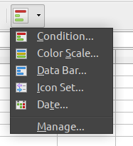
Figure 10: Conditional formatting toolbar icon
Tip
Although each condition type can be accessed using a different option in the Format > Conditional menu of the Menu bar, the five variants of the Conditional Formatting dialog shown in Figures 14 to 18 are not distinct. Once the dialog is open you can create conditions of all types without interacting with the Menu bar. For example, you might create Condition 1 to select a cell style to be used if the cell takes a certain value (Condition 1 is of type “Condition”). You might then press the Add button to create Condition 2 by selecting All Cells in the condition’s upper left drop-down and then selecting Data Bar in the adjacent drop-down (Condition 2 is of type “Data Bar”). You might then press the Add button to create Condition 3 by selecting Date is in the condition’s upper left drop-down (Condition 3 is of type “Date”). In this way you can create many conditions of different types to control the conditional formatting of the selected cells.
The Condition dialog is the starting point when using conditional formatting. Here you can define what formats to use to highlight any data in the spreadsheet that meets the conditions you have defined.
Applies the selected style to the cell or cell range controlled by the condition set in the drop down list. The formatting is applied to each cell individually and the condition may depend on other cells values of the selected range. Valid conditions are described in tables 1, 2 and 3.
Figure 11: Conditional Formatting dialog – Cell value
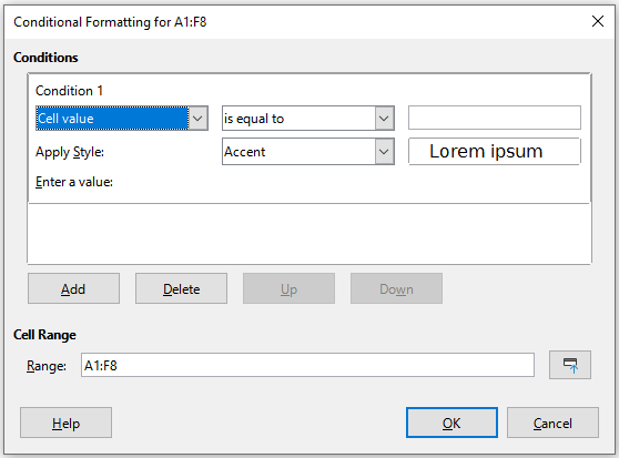
Table 1: Conditions for number and text in cells
Note on text conversion conditions
The condition applies to the internal text conversion of the cell contents. Numeric values are compared with their equivalent text representation. Numeric cell formats (currency, scientific, user-defined ... ) are not considered for comparisons.
Table 2: Conditions for number-only cell values
Note on AVERAGE function in conditions
The average function ignores any text or empty cell within a data range. If you suspect wrong results from this function, look for text in the data ranges. To highlight text contents in a data range, use the Value highlighting feature above.
Table 3: Conditions for errors in cells
Use Color Scale to set the background color of cells depending on the values of the data in those cells. Color Scale can only be used when All Cells has been selected for the condition. You can use either two or three colors for the color scale or gradient.
Figure 12: Conditional Formatting dialog – Color Scale
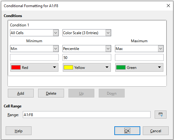
The Color Scale (2 entries ) requires the definition of the colors for the minimum and the maximum values in the range. These two values can be calculated in several ways:
Min (Max): the minimum (maximum) value of the range.
Percentile: A percentile is each of the 99 values which divide the sorted data in 100 equal parts, so that each part represents 1/100 of the sample population. A percentile return the value for a data series going from the smallest to the largest value in a set of data. For P = 25, the percentile means the first quartile. P = 50 is also the MEDIAN of the data set. Enter the percentile value in the text box just below. Valid values are from 0 to 100.
Value: a fixed value set for the minimum (maximum) color. Enter the value in the text box just below.
Percent: a fixed value representing the percentage of the minimum (maximum) of the length defined by minimum and maximum values in the range. A minimum of 10% selects the values below 10% of the segment [Min,Max]. A maximum of 80% select values above 80% of the segment [Min,Max]. Valid values are from 0 (zero) to 100. Do not enter a percent (%) sign.
Formula: A formula expression starting with the equal sign (=) that calculates the numeric value for the minimum (maximum) colors. Values can be numbers, dates or time. Enter the formula expression in the text box just below.
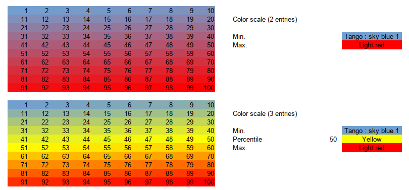
Figure 13: Color scale with 2 and 3 colors
The Color scale (3 entries) allows a third color for an intermediate data value. The third color can be defined as for the Color scale (2 entries) above and with two more options:
Min, Max: The minimum (maximum) value of the range.
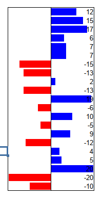
Data bars provide a graphical representation of data in the spreadsheet. The graphical representation is based on the values of data in a selected range. Click on More Options in the Conditional Formatting dialog to define how the data bars will look. Data bars can only be used when All Cells has been selected for the condition.
Figure 14: Conditional Formatting dialog – Data Bar
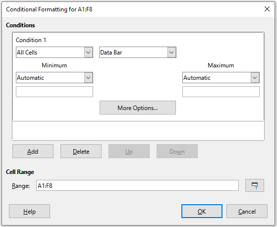
To format all cells with data bars, you must set the minimum and maximum values of the data range. The condition options are the same as the Color Scale above with the addition of:
Automatic: Automatically sets the and maximum value based on the values in the data set.
Figure 15: Data bars
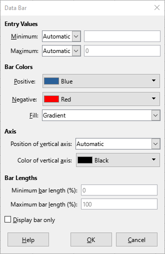
Click on the More Options button to select attributes of the data bars. The Data Bar dialog opens (Figure 16):
Entry values
Bar Colors
Gradient: set a color scale between the color of positive (negative) values and white.
Color: use the positive (negative) color for the entire data bar, no fade out gradient (Figure 15).
Axis
Automatic: position the vertical axis in the middle of the maximum and minimum values.
Middle: set the vertical axis in the middle of the column (Figure 15).
None: do not display a vertical axis.
Bar Lengths
Display bars only
Figure 16: Data bars options
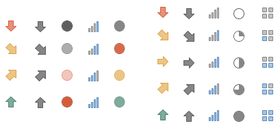
Icon sets display an icon next to the data in each selected cell to give a visual representation of where the cell data falls within the defined range that you set. The icon sets available include colored arrows, gray arrows, colored flags, colored signs, symbols, bar ratings, and quarters (Figure 19 and Figure 20). Icon sets can only be accessed when the Conditional Formatting dialog has been opened and All Cells has been selected for the condition (Figure 17).
Figure 17: Conditional Formatting dialog – Icon Set
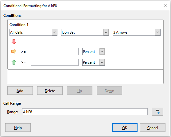
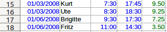
Figure 18 show the icon set used in conditional formatting to show the evolution of data in two datasets.
Figure 18: Arrows icon set used to indicate evolution in data
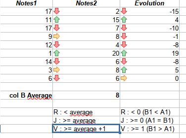
Figure 19: Icon sets with 3 icons

Figure 20: Icon sets with 4 and 5 icons
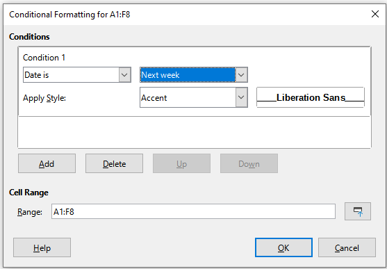
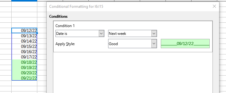
Date applies a defined style depending on a date range chosen in the drop-down menu. Date range options are formed by applying This, Last, and Next adjectives to the available periods for Day, Week, Month, or Year with. Last 7 days is another option available. Examples include Tomorrow (the word for next day), Last 7 days, This week, Next month, Last year.
Figure 21: Conditional Formatting dialog - Date
Note
The start and end of the week is locale dependent (set in Tools > Options > Language Settings > Languages).
Figure 22 Condition for dates in next week.
Applies the selected style to the cell when the formula expression in the text box in the right is not zero.
The formula is expressed similar to a test condition evaluating to TRUE or FALSE.
Figure 23 shows different cell styles applied based on conditions for dates before and after the current date. The formulae are expressed in Table 4.
Figure 23 Conditions to set current, past and future dates using formulas
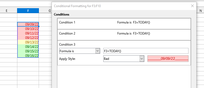
Table 4: Current, past and future deadlines with formulas
|
Deadlines |
Formula is |
Style applied |
|
Current date |
F3 = TODAY() |
"Neutral" |
|
Past date |
F3 < TODAY() |
"Bad" |
|
Future date |
F3 > TODAY() |
"Good" |
To see all the conditional formatting defined in the spreadsheet and any styles used:
1) Go to Format > Conditional > Manage on the Menu bar to open the Manage Conditional Formatting dialog (Figure 24).
Figure 24: Manage Conditional Formatting dialog
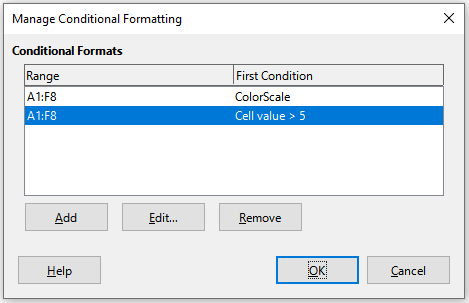
2) Select a range in the Range list and click Edit to redefine the conditional formatting.
3) Select a range in the Range list and click Remove to delete the conditional formatting. The deletion is immediate with no confirmation.
4) Select Add to create a new definition of conditional formatting.
5) Click OK to save the changes and close the dialog.
To apply the style used for conditional formatting to other cells later:
1) Click one of the cells that has been assigned conditional formatting and copy the cell to the clipboard.
2) Select the cells that are to receive the same formatting as the copied cell.
3) Go to Edit > Paste Special > Paste Special on the Menu bar, or right-click and select Paste Special > Paste Special in the context menu, or press Ctrl+Shift+V, to open the Paste Special dialog (Figure 24 above).
4) Make sure that only Formats is selected and click OK to paste the conditional formatting into the cell.
In Calc you can hide elements so that they are neither visible on a computer display nor printed when a spreadsheet is printed. However, hidden elements can still be selected for copying if you select the elements around them; for example, if column B is hidden, it is copied when you select to copy columns A to C. When you require a hidden element again, you can reverse the process and show the element.
Select Sheet > Hide Sheet on the Menu bar, or right-click on the sheet tab for the sheet to be hidden and select Hide Sheet in the context menu. There must always be one sheet that is not hidden.
1) Select a cell in the row or column you want to hide.
2) Go to Format on the Menu bar and select Rows or Columns.
3) Select Hide from the menu and the row or column can no longer be viewed or printed.
4) Alternatively, right-click on the row or column header and select Hide Rows or Hide Columns in the context menu.
Tip
To enable/disable a visual indicator of hidden columns and rows, go to View > Hidden Row/Column Indicator.
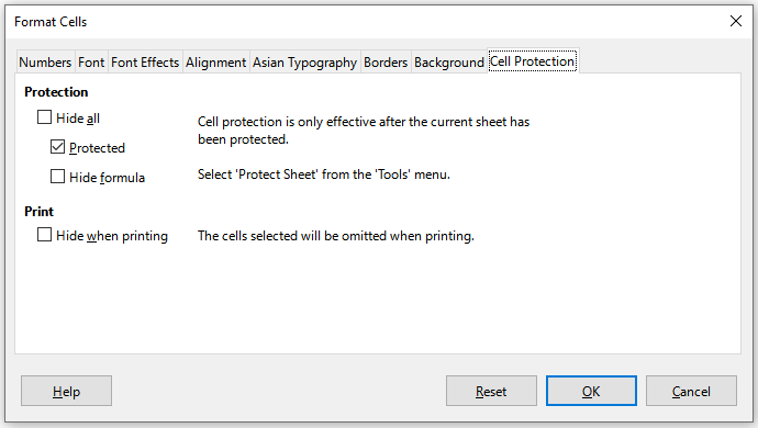
Hiding individual cells is more complicated. First, you need to define the cells as protected and hidden; then you need to protect the sheet:
1) Select the cells you want to hide.
2) Go to Format > Cells on the Menu bar, or right-click and select Format Cells in the context menu, or press Ctrl+1, to open the Format Cells dialog (Figure 25).
3) Click the Cell Protection tab and select an option for hiding and printing the cells.
4) Click OK to save the changes and close the dialog.
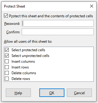
5) Go to Tools > Protect Sheet on the Menu bar, or right-click on the sheet tab and select Protect Sheet in the context menu, to open the Protect Sheet dialog (Figure 26).
6) Select Protect this sheet and the contents of protected cells.
7) Create a password and then confirm the password.
8) Select or deselect the options in the Allow all users of this sheet to area so that users can select protected or unprotected cells.
9) Click OK to save the changes and close the dialog.
Figure 25: Format Cells dialog – Cell Protection tab
Note
When content in cells is hidden, it is only the content contained in the cells that is hidden and the protected cells cannot be modified. The blank cells remain visible in the spreadsheet.
Figure 26: Protect Sheet dialog
Select Sheet > Show Sheet on the Menu bar, or right-click on any sheet tab and select Show Sheet in the context menu. Choose which hidden sheets to show from the list on the Show Sheet dialog. If there are no hidden sheets, the Show Sheet option will not appear in the context menu and will be grayed on the Menu bar.
1) Select the rows or columns on each side of the hidden row or column.
2) Go to Format on the Menu bar and select Rows or Columns. Select Show in the menu and the row or column will be displayed and can be printed.
3) Alternatively, right-click on a row or column header and select Show Rows or Show Columns in the context menu.
1) Go to Tools > Protect Sheet on the Menu bar, or right-click on the sheet tab and select Protect Sheet in the context menu, to open the Protect Sheet dialog (Figure 26).
2) Enter the password to unprotect the sheet and click OK.
3) Go to Format > Cells on the Menu bar, right-click and select Format Cells in the context menu, or press Ctrl+1, to open the Format Cells dialog (Figure 25).
4) Click the Cell Protection tab and deselect the hide options for the cells. Click OK.
Note
When protecting a sheet using the Protect Sheet dialog, you can leave the password fields blank. In this case, the Protect Sheet dialog is not presented at step ) above and step ) is not necessary.