Getting Started Guide 24.8
This document is Copyright © 2024 by the LibreOffice Documentation Team. Contributors are listed below. You may distribute it and/or modify it under the terms of either the GNU General Public License (http://www.gnu.org/licenses/gpl.html), version 3 or later, or the Creative Commons Attribution License (http://creativecommons.org/licenses/by/4.0/), version 4.0 or later.
All trademarks within this guide belong to their legitimate owners.
To this edition
Please direct any comments or suggestions about this document to the Documentation Team’s forum at https://community.documentfoundation.org/c/documentation/loguides/ (registration is required) or send an email to: loguides@community.documentfoundation.org.
Note
Everything you send to a mailing list or forum, including your email address and any other personal information that is written in the message, is publicly archived and cannot be deleted.
Published August 2024. Based on LibreOffice 24.8 Community.
Other versions of LibreOffice may differ in appearance and functionality.
Some keystrokes and menu items are different on macOS from those used in Windows and Linux. The table below gives some common substitutions for the instructions in this book. For a more detailed list, see the application Help.
|
Windows or Linux |
macOS equivalent |
Effect |
|
Tools > Options |
LibreOffice > Preferences |
Access setup options |
|
Right-click |
Control+click and/or right-click depending on computer setup |
Open a context menu |
|
Ctrl (Control) |
⌘ (Command) |
Used with other keys |
|
Alt |
⌥ (Option) or Alt, depending on keyboard |
Used with other keys |
|
F11 |
⌘+T |
Open Styles deck in Sidebar |
Calc is the spreadsheet component of LibreOffice. You can enter data (usually numerical) in a spreadsheet and then manipulate this data to discover results.
Other features provided by Calc include:
Functions, which can be used to create formulas to perform complex calculations on data.
Database functions, to arrange, store, and filter data.
Data statistics tools, to perform complex data analysis.
Dynamic charts, including a wide range of 2D and 3D charts.
Macros, for recording and executing repetitive tasks; scripting languages supported include LibreOffice Basic, Python, BeanShell, and JavaScript.
Ability to open, edit, and save Microsoft Excel spreadsheets.
Import and export of spreadsheets in multiple formats, including HTML, CSV, PDF, and DIF.
Seamless collaboration with other users by sharing spreadsheets.
Simple wildcards such as the asterisk (*), question mark (?), and tilde (~) from other spreadsheet applications are recognized by Calc in formula expressions.
By default, Calc uses its own formula syntax, referred to as Calc A1, rather than the default Excel A1 syntax used by Microsoft Excel. Calc will translate seamlessly between the two. However, if you are familiar with Excel you may wish to change the default syntax by going to Tools > Options > LibreOffice Calc > Formula and choosing Excel A1 or Excel R1C1 in the Formula syntax drop-down menu.
For more information on formula syntax, see Chapter 8, Using Formulas and Functions, in the Calc Guide.
Microsoft Office uses Visual Basic for Applications (VBA) code, and LibreOffice uses Basic code based on the LibreOffice API. Although the programming languages are the same, the objects and methods are different and therefore not entirely compatible.
LibreOffice can run some Excel Visual Basic scripts if you enable this feature at Tools > Options > Load/Save > VBA Properties.
If you want to use macros written in Microsoft Excel using the VBA macro code in LibreOffice, you must first edit the code in the LibreOffice Basic IDE editor.
For more information, refer to Chapter 13, Macros, in the Calc Guide.
For many functions, Calc follows the OpenFormula standard defined in the Recalculated Formula (OpenFormula) Format part of the Open Document Format for Office Applications (OpenDocument) standard, which can be accessed at the OASIS website (https://www.oasis-open.org/). Calc’s general support for OpenFormula leads to a level of inherent compatibility with the function set of any other spreadsheet application that follows the same standard. Note that there are some functions within Calc that are not in accordance with OpenFormula, but many of these are included specifically to improve the exchange of files between Calc and Microsoft Excel.
Calc uses spreadsheets, which consist of a number of individual sheets. Each sheet contains cells arranged in rows and columns, and each cell is identified by its row number and column letter.
Cells hold the individual elements – text, numbers, formulas, and so on – that make up the data to display and manipulate.
Each spreadsheet can have up to 10,000 sheets, and each sheet can have a maximum of 1,048,576 rows and a maximum of 16,384 columns.
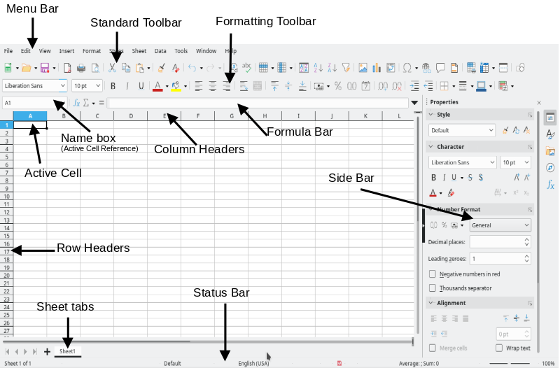
When Calc is started, the main window opens (Figure 1). The parts of this window are described below. You can show or hide many of the parts as desired, using the View menu on the Menu bar.
Note
By default, Calc’s commands are grouped in menus and toolbars, as described in this chapter. In addition, Calc provides other user interface variations, displaying contextual groups of commands and contents. For more information, see Chapter 16, User Interface Variants, in the Calc Guide.
The Title bar, located at the top, shows the name of the current spreadsheet. When a spreadsheet is newly created from a template or a blank document, its name is Untitled X, where X is a number. When you save a spreadsheet for the first time, you are prompted to enter a name of your choice.
Under the Title bar is the Menu bar. When you select one of the menu items, a sub-menu drops down to show commands. You can also customize the Menu bar; see Chapter 13, Customizing LibreOffice, for more information.
Most of the menus are similar to those in other components of LibreOffice, although the specific commands and tools may vary. The menus specific to Calc are Sheet and Data; in addition, several important data analysis tools are found in the Tools menu and the View menu contains several options that are of specific interest to Calc users.
Sheet
Figure 1: Calc main window
Data
Tools
View
In a default LibreOffice installation, the top toolbar under the Menu bar is called the Standard toolbar. It is consistent across all LibreOffice applications. For more information about toolbars, see Chapter 1, LibreOffice Basics.
The Formula bar (Figure 2) is located at the top of the cell grid in the Calc workspace. It is permanently docked in this position and cannot be used as a floating toolbar. However, it can be hidden or made visible by going to View > Formula Bar on the Menu bar.
Figure 2: Formula bar

From left to right, the Formula bar includes the following:
Name Box
Function Wizard
Select Function
Figure 3: Select Function drop-down
Formula
Input line
You can also directly edit the contents of a cell by double-clicking on the cell. When you enter or edit data in a cell, the Select Function and Formula icons change to Cancel and Accept icons.
Note
In a spreadsheet, the term “function” covers much more than just mathematical functions. See Chapter 8, Using Formulas and Functions, in the Calc Guide for more information.
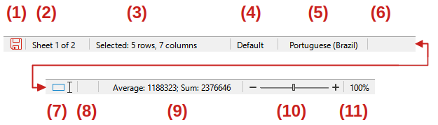
The Status bar (Figure 4) provides information about the spreadsheet as well as quick and convenient ways to change some of its features. Most of the fields are similar to those in other components of LibreOffice. See Chapter 1, LibreOffice Basics, for more information.
Figure 4: Status bar
|
|
|
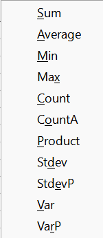
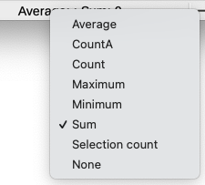
The Status bar can allow you to do quick math operations on selected cells. You can view the calculated average and sum, count of elements, and more on the selection by right-clicking over the Cell/Object Information area and selecting the operations you want to display in the Status bar (Figure 5).
Figure 5: Selecting math operations on Status bar
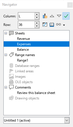
The Sidebar (View > Sidebar or Ctrl+F5) is located on the right-hand side of the window. It is similar to the Sidebar in Writer (shown in Chapter 1 and Chapter 2 of this book) and consists of five decks: Properties, Styles, Gallery, Navigator, and Functions. Each deck has a corresponding icon on the Tab panel on the right-hand side of the Sidebar, allowing you to switch between them. The decks are described below.
Properties
Styles, Gallery, Navigator
Functions
The main section of the Calc workspace displays the cells in the form of a grid. Each cell is formed by the intersection of one column and one row in the spreadsheet.
At the top of the columns and the left of the rows are a series of header boxes containing letters and numbers. The column headers use alphabetic characters beginning at A and go on to the right (to column XFD). The row headers use numerical characters starting at 1 and go down.
These column and row headers form the cell references that appear in the Name Box on the Formula bar (Figure 2). If the headers are not visible on the spreadsheet, choose View > View Headers on the Menu bar.
When the mouse pointer lies over the grid of cells, the system default pointer is normally shown (typically an arrow pointer). However, a configuration option is available to switch to using the pointer shape defined in the icon theme (typically a fat cross). For more information, see Chapter 15, Setting up and Customizing, in the Calc Guide.
The active cell is always indicated by highlighting its corresponding column and row header cells. An option is available to highlight the entire row and column of the active cell using a transparent color. This is enabled/disabled using the Tools > Options > LibreOffice Calc > View > Column/Row highlighting and View > Column/Row Highlighting options on the Menu bar.
Each Calc spreadsheet can contain multiple sheets, which are displayed as tabs at the bottom of the spreadsheet window. By default, each new spreadsheet is created with one sheet named Sheet1 and you can create additional sheets as needed. The tab for the active sheet is highlighted and you can select multiple sheets by holding down the Ctrl key while clicking on the sheet tabs.
To change the default name for a sheet (Sheet1, Sheet2, and so on), right-click on a sheet tab and select Rename Sheet in the context menu, to open the Rename Sheet dialog where you can type a new name for the sheet. You can also access the Rename Sheet dialog by double-clicking on the sheet tab or going to Sheet > Rename Sheet on the Menu bar.
To change the color of a sheet tab, right-click on the tab and select Tab Color in the context menu to open the Tab Color dialog. Select a color and click OK. You can also access the Tab Color dialog by going to Sheet > Sheet Tab Color on the Menu bar. To add new colors to this color palette, see Chapter 13, Customizing LibreOffice.
A comma-separated values (CSV) file contains data in tabular format. In many cases, CSV files contain data exported from a database, resulting in a file in which each line corresponds to a record from a table or query. You can import such data into Calc for futher analysis and charting. A CSV file stores data in a text format, separating values with a specific delimiter character. The delimiter is often a comma but may be a semicolon, a vertical bar, or any other character. Before you open a CSV file in Calc, make sure you know which character is the delimiter. Each line in a CSV file represents a row in a spreadsheet.
To open a CSV file in Calc:
Choose File > Open on the Menu bar, click the Open icon on the Standard toolbar, or press Ctrl+O, and then locate the CSV file. Most CSV files have the extension .csv but some CSV files may have a .txt extension.
Select the file and click Open.
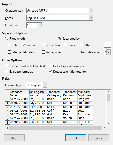
On the Text Import dialog (Figure 6), select the required options for importing the CSV file into the Calc spreadsheet. For details about these options, see Chapter 1, Introduction, in the Calc Guide.
Figure 6: Text Import dialog
Tip
CSV files from different sources may adopt various formats. As you select and deselect options in the upper part of the Text Import dialog, use the preview area in the lower part of the dialog to verify that the layout of the imported data is as expected.
Click OK to import the file.
Caution
Know how your CSV file is formatted before you open it in Calc. Not knowing how the CSV is structured is a source for errors and miscalculations.
For information on how to save files manually or automatically, see Chapter 1, LibreOffice Basics. Calc can save spreadsheets in a range of formats and also export spreadsheets to PDF and XHTML file formats or JPEG, PNG, and WEBP image formats; see Chapter 7, Printing, Exporting, Emailing, and Signing, in the Calc Guide for more information.
You can save a spreadsheet in another format:
Save the spreadsheet in Calc spreadsheet file format (*.ods).
Select File > Save As on the Menu bar to open the Save As dialog. You can also open this dialog by pressing the Ctrl+Shift+S keyboard shortcut, or by clicking the arrowhead icon to the right of the Save icon on the Standard toolbar and selecting Save As in the drop-down menu.
Select the folder where you want to save the file.
In the File name field, enter a new file name for the spreadsheet.
In the Save as type drop-down list, select the type of spreadsheet format you want to use.
If Automatic file name extension is present and selected, the correct file extension for the spreadsheet format you have selected will be added to the file name.
Click Save.
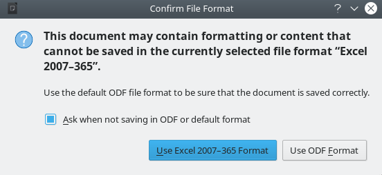
When a spreadsheet file is saved in a format other than .ods, by default the Confirm File Format dialog opens (Figure 7). Click Use [xxx] Format to continue saving in your selected spreadsheet format or click Use ODF Format to save the spreadsheet in Calc .ods format. If you uncheck Ask when not saving in ODF or default format, this dialog no longer appears when saving in another format (the same option can also be found at Tools > Options > Load/Save > General > Warn when not saving in ODF or default format).
Figure 7: Confirm File Format dialog
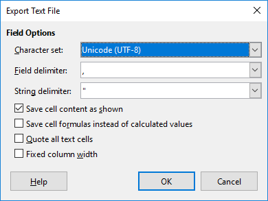
If you select Text CSV (*.csv) format for your spreadsheet, the Export Text File dialog (Figure 8) opens. Here you can set the CSV format for your file, including the character set, the field delimiter, and the string (text) delimiter.
Figure 8: Export Text File dialog for CSV files
Note
Once you have saved a spreadsheet in another format, all changes you make to the spreadsheet will be in that format. If you want to go back to working with a *.ods version, you must save the file as a *.ods file.
Tip
To have Calc save spreadsheets by default in a file format other than .ods, go to Tools > Options > Load/Save > General. In the Default File Format and ODF Settings area, select Spreadsheets (Calc) in Document type, then in Always save as, select your preferred file format.
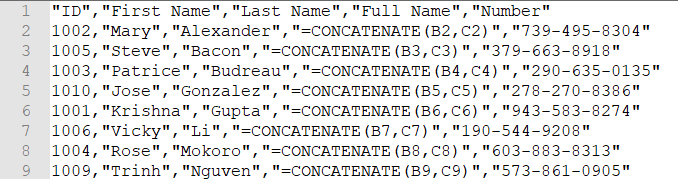
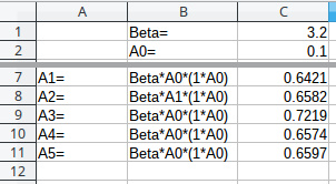
Calc can export raw data and calculated data into a CSV file. Figure 9 contains an example of data for export, and Figure 10 shows the resulting CSV file.
The steps to export are:
Save the spreadsheet in Calc spreadsheet file format (*.ods), for backup purposes.
Select the sheet to be written as a CSV file.
Go to View > Formula on the Menu bar. Alternatively, go to Tools > Options > LibreOffice Calc > View on the Menu bar, check the Formulas option in the Display area, and click OK.
Select File > Save As on the Menu bar to open the Save As dialog. You can also open this dialog by pressing the Ctrl+Shift+S keyboard shortcut, or by clicking the arrowhead icon to the right of the Save icon on the Standard toolbar and selecting Save As in the drop-down menu.
Select the folder where you want to save the file.
In the File name field, enter a new file name for the CSV file.
In the Save as type drop-down list, select Text CSV (*.csv).
If Automatic file name extension is present and selected, the correct file extension for the spreadsheet format you have selected will be added to the file name.
Click Save.
From the Export Text File dialog (Figure 8) that appears, select the required options, and click OK.
Figure 9: Exporting raw and calculated values
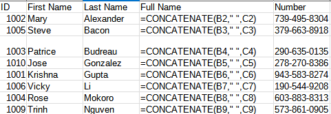
Figure 10: CSV file containing raw and calculated values
If you need to export a range selection or a selected group of shapes (images) into a graphics format, do the following
Select the cell range or the group of shapes, then select File > Export.
In the Export dialog, type a name for the image, select the graphics file format (PNG, JPG, or WEBP), and mark the Selection checkbox.
Click Save.
If necessary, Calc may give you additional options to configure the settings associated with the graphics format.
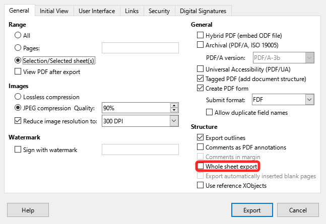
If you need to view an entire sheet, Calc can export a sheet as a PDF in one page.
The steps to export the contents to one page:
On the Menu bar, select File > Export as PDF.
On the General tab of the PDF Options dialog (Figure 11), select the option Whole sheet export.
Click the Export button, and choose a location for the PDF.
Figure 11: Exporting sheets to PDF as one page
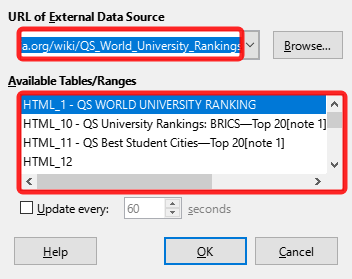
Calc can import data from HTML linking to an external data source with web query. You can filter or choose the table to import by HTML caption:
Position the cursor in the cell where you want the new content to be imported.
Choose Sheet > External Links to open the External Data dialog (Figure 12).
Enter the URL of the HTML document or the name of the spreadsheet, then press Enter. You can also click the Browse button to open a file selection dialog.
In the Available Tables/Ranges list box, select the named ranges or tables you want to insert. You can also specify that the ranges or tables can be updated every n seconds. These tables are now listed in the order they appear in the source. Click OK to finish.
Figure 12: Link to external data
Calc provides many ways to navigate within a spreadsheet, including methods for moving from cell to cell and sheet to sheet.
When a cell is selected or in focus, a colored rectangle is drawn around the cell. When a group of cells is selected, the background of the cell area is colored. The colors depend on the operating system being used and how you have set up LibreOffice.
Home moves the cell focus to the start of a row. Ctrl+Home moves the cell focus to the first cell in the sheet, A1.
The result of pressing End or Ctrl+End depends on the data contained in the sheet. To explain these key presses, it is helpful to define Rmax as the highest numbered row in the sheet that contains any data and Cmax as the rightmost column in the sheet that contains any data. Press End to move the cell focus along the current row to the cell in column Cmax. Press Ctrl+End to move the cell focus to the cell at the intersection of row Rmax and column Cmax. Note that in either case, the newly focused cell may not contain any data.
Page Down moves the cell focus down one complete screen display.
Page Up moves the cell focus up one complete screen display.
Figure 13: Calc Navigator
Each sheet in a spreadsheet is independent of the other sheets, though references can create links between one sheet to another. To navigate between sheets in a spreadsheet:
If your spreadsheet contains multiple sheets, then some of the sheet tabs may be hidden. If this is the case:
Using the four arrowhead buttons to the left of the sheet tabs can move the tabs into view (Figure 14).
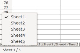
Right-clicking on any of these buttons, or the adjacent + button, opens a context menu where you can select a specific sheet (Figure 15).
Figure 14: Navigating sheet tabs
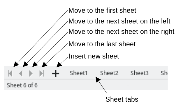
Figure 15: Right-click any active arrow button
Note
When you insert a new sheet into a spreadsheet, Calc automatically uses the next number in the numeric sequence to construct a name. To improve navigation, rename sheets in a spreadsheet to make them more recognizable.
You can navigate a spreadsheet using the keyboard, by pressing a key or a combination of keys. See Chapter 1, Introduction, and Appendix A, Keyboard Shortcuts, in the Calc Guide for the keys and key combinations you can use for spreadsheet navigation in Calc.
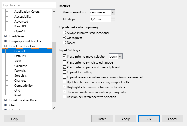
You can customize the behavior of the Enter key by going to Tools > Options > LibreOffice Calc > General on the Menu bar and using the upper three options in the Input Settings area (Figure 16).
Press Enter to move selection: check this option to choose the direction that the cell focus moves after you press the Enter key. Select the required direction of movement in the adjacent drop-down menu (Down, Right, Up, or Left).
Press Enter to switch to edit mode: checking this option causes Enter to open the highlighted cell for editing. Uncheck to make the Enter key select the adjacent cell in the direction of movement defined by the Press Enter to move selection option.
Press Enter to paste and clear clipboard: checking this option causes Enter to paste the content of the clipboard to the highlighted cell, subsequently clearing the clipboard.
Figure 16: Customizing the Enter key
Click in the cell. You can verify your selection by looking in the Name Box on the Formula bar (Figure 2).
A range of cells can be selected using the keyboard or the mouse.
To select a range of cells with the mouse:
Click in a cell.
Press and hold down the left mouse button.
Move the mouse to highlight the desired block of cells, then release the mouse button.
To select a range of cells using the mouse, but without dragging:
Click in the cell at one corner of the range of cells.
Hold down the Shift key and click in the opposite corner cell of the block of cells.
Tip
You can choose a contiguous range of cells by clicking the Selection mode area on the Status bar (Figure 4) and selecting Extending selection before clicking in the opposite corner of the range of cells. Once you are done, make sure to change back to Standard selection or you may extend a cell selection unintentionally.
To select a range of cells using the keyboard:
Click in the cell at one corner of the range of cells.
While holding down the Shift key, use the cursor arrows to select the rest of the range.
Tip
You can also directly select a range of cells using the Name Box. Click in the Name Box on the Formula bar (Figure 2). Enter the cell reference for the upper left-hand cell, followed by a colon (:), and then the lower right-hand cell reference. For example, to select the range that would go from A3 to C6, you would enter A3:C6.
To select a range of non-contiguous cells using the mouse:
Select the first cell or range of cells using one of the methods described in the previous paragraphs.
Move the cursor to the start of the next range or single cell.
Hold down the Ctrl key and click or click-and-drag to select another range of cells to add to the first range.
Repeat as necessary.
Tip
You can choose non-contiguous ranges of cells by clicking the Selection mode area on the Status bar (Figure 4) and selecting Adding selection. Click or click-and-drag to select ranges of cells to add to the selection.
To select a single column, click on the column header (Figure 1). To select a single row, click on the row header.
To select multiple columns or rows that are contiguous:
Click on the header of the first column or row in the group.
Hold down the Shift key.
Click on the header of the last column or row in the group.
To select multiple columns or rows that are not contiguous:
Click on the header of the first column or row in the group.
Hold down the Ctrl key.
Click on the headers of all subsequent columns or rows while holding down the Ctrl key.
Tip
You can also select rows and columns using options in the Edit > Select menu on the Menu bar (Select Row, Select Column, Select Visible Rows Only, and Select Visible Columns Only).
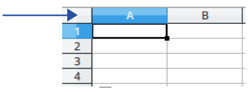
To select the entire sheet, click on the blank rectangular area to the left of the column headers and above the row headers (Figure 17). Alternatively you can press Ctrl+A, press Ctrl+Shift+Space, or go to Edit > Select All on the Menu bar.
Figure 17: Select All box
If you want to make changes to many sheets at once you can select one or multiple sheets in Calc.
Click on the sheet tab for the sheet you want to select. The tab for the selected sheet changes appearance – in the default Calc setup, the tab background color changes to white, the text on the tab changes to bold, and a colored line is drawn along the bottom edge of the tab.
To select multiple contiguous sheets:
Click on the sheet tab for the first desired sheet.
Hold down the Shift key and click on the sheet tab for the last desired sheet.
All tabs between these two selections will change appearance. Any actions that you perform will now affect all the highlighted sheets.
To select multiple non-contiguous sheets:
Click on the sheet tab for the first desired sheet.
Hold down the Ctrl key and click on the sheet tab for the each additional desired sheet.
The selected tabs will change appearance. Any actions that you perform will now affect all the highlighted sheets.
Right-click a sheet tab and choose Select All Sheets in the context menu, or select Edit > Select > Select All Sheets on the Menu bar.
Tip
You can also select sheets using the Select Sheets dialog, accessed by selecting Edit > Select > Select Sheets on the Menu bar.
Using the Sheet menu:
Select the cell location where you want the new column or row inserted.
Go to Sheet on the Menu bar and select either Insert Columns > Columns Before, Insert Columns > Columns After, Insert Rows > Rows Above, or Insert Rows > Rows Below.
Using row and column headers:
Right-click the column or row header where you want the new column or row inserted.
Select Insert Columns Before, Insert Columns After, Insert Rows Above, or Insert Rows Below in the context menu.
To insert multiple columns or rows at once:
Highlight the required number of columns or rows by holding down the left mouse button on the first one and then dragging across the required number of identifiers.
Proceed as for inserting a single column or row above.
To hide columns or rows:
Select cells in the rows or columns you want to hide.
Go to Format on the Menu bar, select Rows or Columns, and select Hide in the submenu. Alternatively, right-click on selected row or column headers and select Hide Rows or Hide Columns in the context menu.
To show hidden columns or rows:
Select cells in the rows or columns on each side of the hidden rows or columns.
Go to Format on the Menu bar, select Rows or Columns, and select Show in the submenu. Alternatively, right-click on selected row or column headers and select Show Rows or Show Columns in the context menu.
Tip
To see an indicator for hidden columns and rows, enable the View > Hidden Row/Column Indicator option on the Menu bar.
To delete multiple columns or rows, do one of the following:
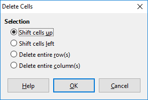
Select a range of cells across the columns or rows you want to delete, right-click and select Delete in the context menu, select Sheet > Delete Cells on the Menu bar, or press Ctrl+- to open the Delete Cells dialog (Figure 18). Select Delete entire column(s) or Delete entire row(s) and click OK.
Select a range of cells across the columns or rows you want to delete and select Sheet > Delete Columns or Sheet > Delete Rows on the Menu bar.
Highlight the required columns or rows by holding down the left mouse button on the header of the first one and then dragging across the required number of headers. Then right-click on one of the selected column or row headers and select Delete Columns or Delete Rows in the context menu.
Select the cells you want to delete. Choose the Sheet > Delete Cells command, press Ctrl+-, or right-click on a cell and select Delete in the context menu.
When the Delete Cells dialog (Figure 18) appears, select the appropriate option and click OK.
Figure 18: Delete Cells dialog
If you need to insert a new sheet after the last sheet in a spreadsheet without opening the Insert Sheet dialog, click the Add Sheet (+) icon next to the sheet tabs. After clicking on the icon, the the new sheet appears with an automatically allocated name.
The Insert Sheet dialog (Figure 19) provides greater flexibility and is accessed by one of the following methods:
Figure 19: Insert Sheet dialog

Select the sheet where you want to insert a new sheet, then go to Sheet > Insert Sheet on the Menu bar.
Right-click on the sheet tab where you want to insert a new sheet and select Insert Sheet in the context menu.
The Insert Sheet dialog is used to position the new sheet, create multiple sheets, name the new sheet, or select a file containing the data to be inserted into the new sheet.
You can move a sheet to a different position within the same spreadsheet, by clicking on the sheet’s tab and dragging it to a new position before releasing the mouse button. You can copy a sheet within the same spreadsheet, by holding down the Ctrl key, clicking on the sheet tab, and dragging it to its required position before releasing the mouse button. You can also copy a sheet by right-clicking the sheet’s tab and selecting Duplicate Sheet in the context menu, or by going to Sheet > Duplicate Sheet on the Menu bar.
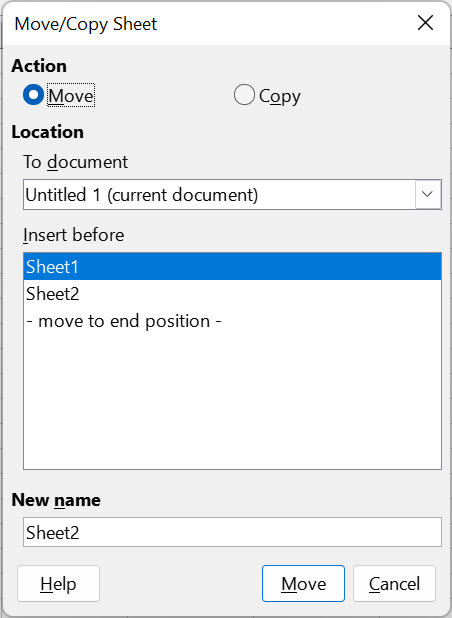
The Move/Copy Sheet dialog (Figure 20) provides greater flexibility and, in particular, allows you to move or copy a sheet into a different spreadsheet.
To access the Move/Copy Sheet dialog, right-click on the sheet tab you wish to move or copy and then select Move or Copy Sheet in the context menu, or go to Sheet > Move or Copy Sheet on the Menu bar.
In the Action area, select Move to move the sheet or Copy to copy the sheet.
Select the spreadsheet where you want the sheet to be placed in the To document drop-down list.
In the Insert before list, choose the position in the target spreadsheet where you want to place the sheet.
Enter a name in the New name box if you want to rename the sheet after it is moved or copied. If you do not enter a name, Calc automatically generates one.
Click Move or Copy to confirm the move or copy and close the dialog.
Figure 20: Move/Copy Sheet dialog
Caution
When you move or copy a sheet to another spreadsheet, a conflict may occur with formulas linked to other sheets in the previous location.
If you need to hide one or more sheets, first select the sheets. Then right-click on one of the selected sheet tabs and select Hide Sheet in the context menu, or go to Sheet > Hide Sheet on the Menu bar. It is not possible to hide the last visible sheet.
To display hidden sheets, right-click on any sheet tab and select Show Sheet in the context menu, or go to Sheet > Show Sheet on the Menu bar. Calc displays the Show Sheet dialog, listing all hidden sheets. Select the hidden sheets to be displayed again and then click OK.
It is also possible to hide and show elements within a sheet, as described in various chapters of the Calc Guide.
Every time a new sheet is created without specifying a name, it is automatically named SheetX (where X is an incrementing number allocated by Calc). The first sheet in a new spreadsheet is named Sheet1.
A sheet can be renamed using one of the following methods:
Enter a new name in the Name text box when creating the new sheet using the Insert Sheet dialog (Figure 19).
Right-click on the sheet’s tab and select Rename Sheet in the context menu to open the Rename Sheet dialog.
Select the sheet’s tab and go to Sheet > Rename Sheet on the Menu bar to open the Rename Sheet dialog.
Double-click on the sheet’s tab to open the Rename Sheet dialog.
Note
Sheet names can contain almost any character. Some naming restrictions apply, the following characters are not allowed in sheet names: colon (:), back slash (\), forward slash (/), question mark (?), asterisk (*), left square bracket ([), or right square bracket (]). In addition a single quote (‘) cannot be used as the first or last character of the name. Attempting to rename a sheet with an invalid name will produce an error message.
To delete one or more sheets, first select the sheets (see “Selecting sheets” above). Then right-click on one of the selected sheet tabs and select Delete Sheet in the context menu, or go to Sheet > Delete Sheet on the Menu bar. If any of the selected sheets is not empty, then Calc displays a confirmation dialog stating the number of sheets to be deleted. Click Yes to confirm the deletion. It is not possible to delete all the sheets in a spreadsheet.
Use the zoom function (View > Zoom) to show more or fewer cells in the window when you are working on a spreadsheet. For more about zoom, see Chapter 1, LibreOffice Basics.
If you have long rows or columns of data that extend beyond the viewable area of the sheet, you can freeze selected rows or columns. In this way you can lock rows across the top of a sheet or lock columns down the left of a sheet, so that the frozen data remains displayed as you scroll through the rest of the data. Vertical scrolling does not affect the visibility of data in a frozen row; horizontal scrolling does not affect the visibility of data in a frozen column.
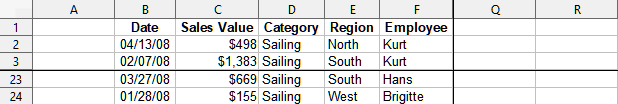
The sheet shown in Figure 21, has frozen rows and columns, which are outlined by heavy lines. Columns A through F and rows 1 through 3 are frozen. The rows between 3 and 23 and the columns between F and Q are scrolled off the page.
Figure 21: Frozen rows and columns
To freeze the first column in a sheet go to View > Freeze Cells > Freeze First Column on the Menu bar, or click the down arrow to the right of the Freeze Rows and Column icon on the Standard toolbar and select Freeze First Column in the drop-down menu.
To freeze the first row in a sheet go to View > Freeze Cells > Freeze First Row on the Menu bar, or click the down arrow to the right of the Freeze Rows and Column icon on the Standard toolbar and select Freeze First Row in the drop-down menu.
To freeze either a set of rows or a set of columns (single or multiple):
Click on the header of the row below all the rows you want to freeze, or click on the header of the column to the right of all the columns you want the freeze.
Right-click on the header and select Freeze Rows and Columns in the context menu, or go to View > Freeze Rows and Columns on the Menu bar, or click the Freeze Rows and Columns icon on the Standard toolbar.
To freeze both a set of rows and a set of columns (single or multiple):
Click in the cell that is immediately below the rows you want to freeze and immediately to the right of the columns you want frozen.
Choose View > Freeze Rows and Columns on the Menu bar, or click the Freeze Rows and Columns icon on the Standard toolbar.
To unfreeze all rows and columns that are currently frozen, do one of the following:
Right-click on any row or column header and choose Freeze Rows and Columns in the context menu.
Select View > Freeze Rows and Columns on the Menu bar.
Click the Freeze Rows and Columns icon on the Standard toolbar.
The heavy lines that indicate frozen rows and columns will disappear.
Calc allows you to view different areas of a sheet simultaneously by splitting the screen into separate sections. Each section provides you with a view of one part of the sheet. This feature is also known as “splitting the window.” The screen can be split horizontally, vertically, or both at once (which would give you up to four sections of the sheet in view at one time). Figure 22 provides an example of a sheet split horizontally into two sections, with the split indicated by the gray separator line located between rows 2 and 7.
This feature is especially useful when a large spreadsheet has one cell containing data that is used by three formulas in different cells. When you the split the screen, you can position the cell containing the number in one section of the view and the cells with formulas in other sections. This makes it easy to see how changing the number in one cell affects each of the formulas.
Figure 22: Split screen example
There are two methods to split a screen either horizontally or vertically. In these cases, you can scroll through each section independently of the other. A horizontal or vertical separator line appears indicating where the split has been placed.
Method 1
To split horizontally, you can right-click on the row header below the row where you want to split and select Split Window in the context menu. Alternatively you can left-click on the row header below the row where you want to split and then go to View > Split Window on the Menu bar or click the Split Window icon on the Standard toolbar.
To split vertically, you can right-click on the column header to the right of the column where you want to split and select Split Window in the context menu. Alternatively you can left-click on the column header to the right of the column where you want to split and then go to View > Split Window on the Menu bar or click the Split Window icon on the Standard toolbar.
Method 2
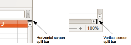
To split horizontally, click on the horizontal split bar at the top of the vertical scroll bar (Figure 23 – left) and drag it down to a position below the row where you want the horizontal split.
To split vertically, click on the vertical split bar at the right of the horizontal scroll bar (Figure 23 – right) and drag it left to a position to the right of the column where you want the vertical split.
There are two methods to split a screen both horizontally and vertically at the same time. Horizontal and vertical separator lines appear indicating where the split has been placed.
Method 1
Click in the cell that is below the row and to the right of the column where you want to split. Go to View > Split Window on the Menu bar or click the Split Window icon on the Standard toolbar.
Method 2
Click on the horizontal split bar at the top of the vertical scroll bar (Figure 23 – left) and drag it down to a position below the row where you want the horizontal split. Then, click on the vertical split bar to the right of the horizontal scroll bar (Figure 23 – right) and drag it left to a position to the right of the column where you want the vertical split.
Figure 23: Split screen bars
To remove a split view, do one of the following:
Double-click on each split line.
Click and drag the split lines back to their default positions at the ends of the scroll bars.
Go to View on the Menu bar and deselect Split Window.
Right-click on a column or row heading and deselect Split Window in the context menu.
Click the Split Window icon on the Standard toolbar.
Most data entry in Calc is done with the keyboard.
Click in the cell and type the number using the number keys on either the main keyboard or the numeric keypad. By default, Calc right-aligns the numbers in a cell.
To enter a negative number, either type a minus (–) sign in front of the number or enclose the number in parentheses(1234). The negative number will be displayed as follows: –1234.
If a number is entered with leading zeroes (for example, 01481), Calc will drop the leading zeroes by default. To retain a minimum number of characters in a cell when entering numbers and retain the number format, for example 1234 and 0012, use one of two methods to add leading zeroes:
Method 1
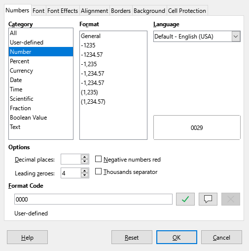
Select the cell that will retain leading zeroes, then access the Format Cells dialog (Figure 24) by doing one of the following:
Right-click on the selected cell then choose Format Cells in the context menu.
Go to Format > Cells on the Menu bar.
Press Ctrl+1.
Select the Numbers tab and select Number in the Category list.
In the Options area, set the Leading zeroes field to the maximum number of zeroes to display in front of the integer part of the number. If you want to display numbers with four integer digits, enter the value 4. Then any number containing less than four integer digits will have leading zeroes added – for example 12 is displayed as 0012.
Figure 24: Format Cells dialog – Numbers tab
Click OK. The number in the selected cell retains its number format and any formula used in the spreadsheet will treat the entry as a number in formula functions.
Method 2
Select the cell.
On the Sidebar, go to the Properties deck.
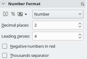
On the Number Format panel (Figure 25), select Number in the drop-down list, and enter the maximum number of zeroes to display in front of the integer part of a number in the Leading zeroes box. Formatting is applied immediately.
Figure 25: Set leading zeroes in Sidebar
Tip
To format numbers with decimal places and prevent a leading zero (for example, “.019” instead of “0.019”), go to the Format code box on the Numbers tab of the Format Cells dialog and then type a period or full stop and add one or more question marks (“?”). Each question mark represents a decimal place. For example, for 3 decimal places, type one period and three question marks [.???] and click OK. Any number with only decimal places will then have no leading zero.
Tip
If a numeric value does not need to be treated as a number in calculations (for example when entering a zip code), you can type an apostrophe (') before the number, for example “'01481”. When you move the cell focus, the apostrophe is hidden, any leading zeroes are retained, and the number is converted to left-aligned text.
Numbers can also be entered as text using one of the following methods:
Method 1
Select the cell which contains the number, then access the Format Cells dialog (Figure 24).
Make sure the Numbers tab is selected, then select Text in the Category list.
Click OK. The number is converted to text and, by default, left-aligned.
Method 2
Select the cell.
On the Sidebar, go to the Properties deck.
On the Number Format panel (Figure 25), select Text in the drop-down list. Formatting is applied to the cell immediately.
Note
You can change how Calc converts strings to numeric values, cell references, dates, and times by going to Tools > Options > LibreOffice Calc > Formula. In the Detailed Calculation Settings area, select Custom (conversion of text to numbers and more). Click the Details button, and then select the proper treatment in the Detailed Calculation Settings dialog. See the system help for more information.
To enter text in a cell, click in the cell and type. By default, text is left-aligned in a cell. Cells can contain several lines of text. If you want to use paragraphs, press Ctrl+Enter to create another paragraph.
If you are entering several lines of text, extend the Input line by clicking on the Expand Formula Bar icon, which is located on the right-hand end of the Formula bar, and then the Input line becomes multi-line. Click the icon again to return the Input line to its single line height.
Select the cell and type the date or time. You can separate the date elements with a slash (/) or a hyphen (–), or use text, for example 10 Oct 2020. The date format automatically changes to the selected format used by Calc.
Note
Tools > Options > Languages and Locales > General > Formats > Date acceptance patterns defines the date patterns that will be recognized by Calc. In addition, every locale accepts input in an ISO 8601 YYYY-MM-DD pattern (for example, 2020-07-26).
When entering a time, separate time elements with colons (for example, 10:43:45) and the time format automatically changes to the selected format used by Calc.
To change the date or time format used by Calc:
With the cell selected, open the Format Cells dialog (Figure 24).
Make sure the Numbers tab is selected, then select Date or Time in the Category list.
Select the date or time format you want to use in the Format list.
Click OK.
If you wish to insert a date, the sheet name, or the document name in a cell as a field, do the following:
Select a cell and double-click to activate edit mode.
Right-click and select Insert Field > Date, Sheet Name, or Document Title in the context menu. The Insert Field sub-menu contains two Date options – use the occurrence located directly above the Sheet Name item. Alternatively you can go to Insert > Field > Date, Sheet Name, or Document Title on the Menu bar.
The fields are updated with the latest information when the spreadsheet is saved or recalculated using the Ctrl+Shift+F9 shortcut or going to Data > Calculate > Recalculate Hard on the Menu bar.
Note
The other Insert Field > Date option and its associated Time option in the context menu insert the current date and time respectively. However, unlike the commands described above, these values are not inserted as fields and will not be updated or recalculated later. Similarly, the Insert > Date and Insert > Time options on the Menu bar do not insert values as fields.
Note
The Document Title commands insert the name of the spreadsheet. They do not insert the title defined on the Description tab of the Properties dialog for the file.
Calc automatically applies many changes during data input using AutoCorrect, unless you have deactivated any AutoCorrect changes. For more information, refer to Chapter 2, Entering and Editing Data, in the Calc Guide. You can also undo any AutoCorrect changes by using Edit > Undo on the Menu bar, pressing the keyboard shortcut Ctrl+Z, or manually by going back to the change and replacing the automatic correction with what you want.
To change how AutoCorrect works, go to Tools > AutoCorrect Options on the Menu bar to display the AutoCorrect dialog (Figure 26):
Figure 26: AutoCorrect dialog
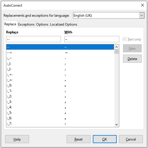
To turn off some or all AutoCorrect features, go to Tools > AutoCorrect Options on the Menu bar and uncheck unwanted features on the Options and Localized Options tabs on the AutoCorrect dialog.
Calc provides multiple tools for removing some of the drudgery from input. The most common tool is to drag and drop the contents of one cell to another with a mouse. Other tools include AutoInput, the Fill tool, selection lists, the Data Entry tool, and the ability to input information into multiple sheets of the same document.
The AutoInput tool in Calc automatically completes entries, based on other entries in the same column. By default, AutoInput is activated in Calc. To turn it off, go to Tools on the Menu bar and deselect AutoInput.
When text is highlighted in a cell, AutoInput can be used as follows:
Press Enter to accept the completion and move to the next cell. Press F2 to accept the completion and move the cursor to the end of the text inside the cell. Clicking outside the cell will accept the completion and select the clicked cell.
When multiple matches continue with the same letters they will appear in the cell after what has already been typed. Press Right Arrow to accept the partial completion and move the cursor to the end of the text inside the cell.
To view more completions that start with the same letters, use the key combinations Ctrl+Tab to scroll forward, or Ctrl+Shift+Tab to scroll backward.
To see a list of all available AutoInput text items for the current column, use the keyboard combination Alt+Down Arrow.
When typing formulas using characters that match function names, a help tip will appear listing the available functions that start with matching characters. AutoInput ignores the case sensitivity of any data you enter.
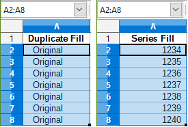
This tool allows you to duplicate existing content or create a series across a range of cells (see examples in Figure 27) using one of the following methods.
Caution
When you are selecting cells to use the Fill tool, make sure that none of the cells contain important data, except for the cell data you want to use. When you use the Fill tool, any data contained in the selected target cells is overwritten.
Method 1
Select one or more cells that contain the contents you want to copy or start the series from.
Drag the mouse pointer to fill the cells in any direction you desire, or hold down the Shift key and click in the last cell you want to fill.
Go to Sheet > Fill Cells on the Menu bar and select the direction in which you want to copy or create data (Fill Down, Fill Right, Fill Up, Fill Left) or one of the other options (Fill Sheets, Fill Series, Fill Random Number) in the submenu. For more information about the Fill Sheets and Fill Random Number options, see Chapter 2, Entering and Editing Data in the Calc Guide.
Tip
Ctrl+D is an alternative to selecting Sheet > Fill Cells > Fill Down on the Menu bar.
Method 2
Select one or more cells that contain the contents you want to copy or start the series from.
Move the mouse pointer over the small square in the bottom right corner of the selected cells. The mouse pointer will change shape.
Click and drag in the direction you want the cells to be filled. If the original cell contained a number or text from a defined sort list, then a series will be created. However, if the Ctrl button is pressed while dragging, then the original data is copied instead. If the original cell contained any other text, then that text will automatically be copied.
Figure 27: Using the Fill tool
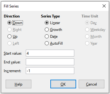
When you select a series fill from Sheet > Fill Cells > Fill Series on the Menu bar, the Fill Series dialog (Figure 28) opens. Here you can select the type of series you want. For more detail about this dialog, see Chapter 2, Entering and Editing Data in the Calc Guide.
Figure 28: Fill Series dialog
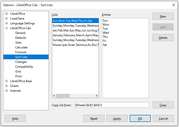
When a fill is initiated and the selected cell contains text, Calc will check if one of your predefined sort lists contains that text. If there is a sort list containing the text, Calc uses the entries in that sort list to fill cells. Go to Tools > Options > LibreOffice Calc > Sort Lists to view your currently defined sort lists.
To define your own sort list, which can later be used as a fill series:
Go to Tools > Options > LibreOffice Calc > Sort Lists to open the Sort Lists dialog (Figure 29). This dialog shows any previously-defined series in the Lists box and the contents of the highlighted list in the Entries box.
Click New and the Entries box is cleared.
Type the series for the new list in the Entries box (one entry per line).
Click Add and the new list will appear in the Lists box.
Click OK to save the new list.
Selection lists are limited to using only text that has already been entered in the same column.
Select a blank cell in a column that contains cells with text entries.
Right-click and select Selection Lists in the context menu, or press Alt+Down Arrow. A context menu appears listing any cell in the same column that either has at least one text character or whose format is defined as text.
Click on the text entry you require and it is entered into the selected cell.
Figure 29: Sort Lists dialog
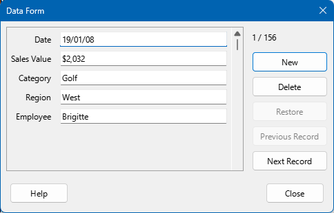
This tool makes table data entry easier in spreadsheets, accelerating intensive manual input. Using the tool you can enter, edit, and delete data records (or rows) and avoid horizontal scrolling when the table has many columns or when some columns are very wide.
To be effective, the data table should have a header row, where the content of each cell is the title of the column. The content of each header cell becomes the label for each data field in the form.
To use the Data Entry Form tool:
Select a header or data cell within the table of data.
Go to Data > Form on the Menu bar.
Calc displays the Data Form dialog (Figure 30), showing the data for the first entry in the data table.
Add, edit, or remove entries from the data table as required.
Click the Close button to close the dialog.
Figure 30: Data Form dialog
You might want to share the same information in the same cell on multiple sheets (for example, to set up standard listings for a group of individuals or organizations). Instead of entering the list on each sheet individually, you can enter the information in several sheets at the same time.
Select the individual sheets where you want the information to be repeated. See the section “Selecting sheets” above for more details.
Enter the information in the cells on the first sheet where you want it to appear and it will be repeated in all the selected sheets.
Caution
This technique automatically overwrites, without any warning, any information that is already in the cells on the selected sheets. Make sure you deselect the additional sheets when you are finished entering information that is going to be repeated before continuing to enter data into the spreadsheet.
When creating a spreadsheet, you may want to restrict users to entering data that is valid and appropriate for the cell. Fill tools and selection lists can handle some types of data, but are limited to predefined information.
To add data validation to a cell, select that cell and use Data > Validity on the Menu bar to define which types of content can be entered in the cell. The Validity tool can:
Define the range of contents that can be entered.
Provide help messages explaining the content rules set up for the cell.
Determine what happens if a user enters invalid content. You can set the cell to refuse invalid content, accept it with a warning, or start a macro when an error is entered.
See Chapter 2, Entering and Editing Data, in the Calc Guide for more information.
Calc has multiple tools for data editing, including the ability to delete data, replace data, and change data.
To completely replace data in a cell, select the cell and type in the new data. The new data will replace the old, but cell formatting will be retained.
Alternatively, select the cell and click in the Input line on the Formula bar (Figure 2), then double-click on the data to highlight it completely and type the new data.
Calc can allow you to edit the contents of a cell without removing all of the data from the cell. For example, changing the phrase “Sales in Qtr. 2” to “Sales rose in Qtr” can be done as follows.
Click in the cell to select it.
Press F2 to switch the cell to edit mode. The cursor is placed at the end of the content in the cell.
Use the keyboard arrow keys to position the cursor where you want to start entering the new data in the cell, then press the Delete key or Backspace key to delete any unwanted data before typing the new data.
When you have finished editing, press the Enter key to save the changes.
Tip
You may want to enable Tools > Options > LibreOffice Calc > General > Press Enter to switch to edit mode. Then, when you press the Enter key in a selected cell, the cell switches to edit mode, eliminating the need to press F2.
Use one of the following methods to prepare for editing cell data:
Double-click on the cell to select it and enter cell edit mode.
Click in the cell to select it and press F2 to enter cell edit mode.
Click in the cell to select it and go to Edit > Cell Edit Mode on the Menu bar to enter cell edit mode.
Click in the cell to select it and then click in the Input line of the Formula bar.
Reposition the cursor to where you want to start editing the data, either in the cell or the Input line.
When you have finished, click away from the cell to deselect it and save the changes.
To copy text, numbers, or formulas to the target cell or cell range:
Select the source cell or cell range and copy the data by pressing Ctrl+C, going to Edit > Copy on the Menu bar, clicking the Copy icon on the Standard toolbar, or right-clicking and selecting Copy in the context menu.
Select the target cell or cell range.
Right-click on the target cell or cell range and select Paste Special in the context menu, then select Unformatted Text, Text, Number, or Formula. Alternatively, use the equivalent submenu items reached from Edit > Paste Special on the Menu bar.
You can also use the Paste Special dialog to paste into another cell selected parts of the data in the original cell or cell range, for example its format or the result of its formula. To do this:
Select the source cell or cell range and copy the data by pressing Ctrl+C, going to Edit > Copy on the Menu bar, clicking the Copy icon on the Standard toolbar, or right-clicking and selecting Copy in the context menu.
Select the target cell or cell range.
Go to Edit > Paste Special > Paste Special on the Menu bar, or press Ctrl+Shift+V, or right-click and select Paste Special > Paste Special in the context menu to open the Paste Special dialog (Figure 31).
Figure 31: Paste Special dialog
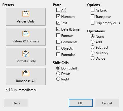
In the preset buttons on the left side of the dialog, you can choose to paste Values Only, Values & Formats, Formats Only, or to Transpose All the data in the target cells. On the right side of the dialog, select the options for Paste, Options, Operations, and Shift Cells. These are described in Chapter 2, Entering and Editing Data, in the Calc Guide.
Click OK to paste the data into the target cell or range of cells and close the dialog.
Tip
To see which combination of options on the right side would apply if one of the buttons in the Presets area is selected, deselect the Run immediately option. With the Run immediately option selected, clicking on a preset button applies that combination of options and closes the dialog.
To delete only the data in a cell or range of cells, without deleting any of the cell formatting, select the cells and then press the Delete key.
To completely delete rows or columns, see the “Deleting columns or rows” section above. To completely delete cells, see the “Deleting cells” section above.
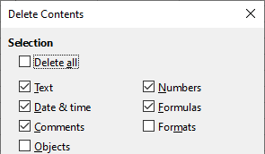
Data and cell formatting can be deleted from a cell at the same time. To do this:
Select a cell or a range of cells.
Press the Backspace key, or right-click in the cell selection and choose Clear Contents in the context menu, or select Sheet > Clear Cells on the Menu bar.
In the Delete Contents dialog (Figure 32), choose any of the options or Delete all.
Click OK.
Figure 32: Delete Contents dialog
Note
All the settings discussed here can be set as a part of the cell style. See Chapter 5, Using Styles and Templates, in the Calc Guide for more information.
Multiple lines of text can be entered into a single cell using automatic wrapping or manual line breaks.
To automatically wrap multiple lines of text in a cell, use one of the following methods:
Method 1
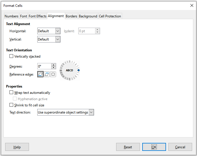
Select the cell and then access the Format Cells dialog (Figure 24).
On the Alignment tab (Figure 33), under Properties, select Wrap text automatically and click OK.
Figure 33: Format Cells dialog – Alignment tab
Method 2
Select the cell.
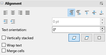
On the Properties deck of the Sidebar, open the Alignment panel (Figure 34).
Select the Wrap text option to apply the formatting immediately.
Figure 34: Wrap text formatting
Method 3
Select the cell.
Click the Wrap Text icon on the Formatting toolbar.
To insert a manual line break in a cell, press Ctrl+Enter. When editing text, double-click the cell, then reposition the cursor to where you want the line break. In the Input line of the Formula bar, you can also press Shift+Enter.
When a manual line break is entered in a cell, the cell row height changes but the cell width does not change and the text may still overlap the end of the cell. You may need to change the cell width manually or reposition the line break.
The font size of the data in a cell can automatically adjust to fit inside cell borders. To do this, select the Shrink to fit cell size option under Properties on the Alignment tab of the Format Cells dialog (Figure 33).
You can select contiguous cells and merge them into one large cell by:
Selecting the range of contiguous cells you want to merge.
Performing one of these steps:
Right-clicking on the selected cells and select Merge Cells in the context menu.
Going to Format > Merge and Unmerge Cells > Merge Cells or Merge and Center Cells on the Menu bar. Using Merge and Center Cells will center align any contents in the cells.
Clicking on the Merge Cells or Merge and Center Cells icon on the Formatting toolbar.
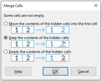
If the cells contain any data, a small dialog (Figure 35) opens, showing choices for moving or hiding data in the hidden cells. Make your selection and click OK.
Caution
Merging cells can lead to calculation errors in formulas used in the spreadsheet.
Figure 35: Merge choices for non-empty cells
You can split a cell that was created from several cells by:
Selecting a merged cell.
Going to Format > Merge Cells > Unmerge Cells on the Menu bar, or right-clicking and selecting Unmerge Cells in the context menu, or clicking on the Unmerge Cells icon on the Formatting toolbar.
Any data in the cell will remain in the first cell. If the hidden cells did have any contents before the cells were merged, then you have to manually move the contents in to the correct cell.
Calc allows you to apply number formats by using icons on the Formatting toolbar. Select the cell, then click the relevant icon to change the number format.
For more control or to select other number formats, use the Numbers tab of the Format Cells dialog (Figure 24):
Apply any of the data types in the Category list to the data.
Select one of the predefined formats in the Format list.
Control the number of decimal places and leading zeroes in the Options area.
Enter a custom format code.
The Language setting controls the local settings for the different formats such as the date format and currency symbol.
Some number formats are available on the sidebar’s Number Format panel of the Properties deck. Click the More Options button to open the Format Cells dialog.
Tip
For consistency in a spreadsheet, use cell styles whenever possible.
To manually select a font and format text for use in a cell:
Select a cell or cell range.
To change the font: click the arrowhead icon to the right of the Font Name box on the Formatting toolbar and select a font in the drop-down menu. A font is temporarily applied on selected cells by hovering or navigating in this menu. The font can also be changed using the Font tab of the Format Cells dialog or the Character panel on the Properties deck of the Sidebar.
To change the font size: click the arrowhead icon to the right of the Font Size box on the Formatting toolbar and select a font size in the drop-down menu. The font size can also be changed using the Font tab of the Format Cells dialog or the Character panel on the Properties deck of the Sidebar.
To change the character format, use one of the following methods:
Click on the Bold, Italic, or Underline icons on the Formatting toolbar.
Press Ctrl+B (bold), Ctrl+I (italic), or Ctrl+U (underline) keyboard shortcuts.
Go to Format > Text on the Menu bar and select Bold, Italic, Single Underline, or Double Underline in the submenu.
Click on the Bold, Italic, or Underline icons on the Character panel on the Properties deck of the Sidebar.
Select Bold, Italic, or Bold Italic in the Style menu on the Font tab of the Format Cells dialog. Select an entry in the Underlining menu on the Font Effects tab of the Format Cells dialog.
To change the horizontal paragraph alignment, do one of the following:
Click on one of the horizontal alignment icons (Align Left, Align Center, or Align Right) on the Formatting toolbar.
Press Ctrl+L (left), Ctrl+E (center), Ctrl+R (right), or Ctrl+J (justified) keyboard shortcuts.
Go to Format > Align Text on the Menu bar and select Left, Centered, Right, or Justified in the submenu.
Click on the Align Left, Align Center, Align Right, or Justified icons on the Alignment panel of the Properties deck on the Sidebar.
Select Left, Center, Right, Justified, Filled, or Distributed in the Horizontal menu on the Alignment tab of the Format cells dialog.
To change the vertical paragraph alignment, do one of the following:
Click on one of the vertical alignment icons (Align Top, Center Vertically, Align Bottom) on the Formatting toolbar.
Go to Format > Align Text on the Menu bar and select Top, Center, or Bottom in the sub-menu.
Click on the Align Top, Center Vertically, or Align Bottom icons on the Alignment panel of the Properties deck on the Sidebar.
Select Top, Middle, Bottom, Justified, or Distributed in the Vertical menu on the Alignment tab of the Format cells dialog.
To change the font color, do one of the following:
Click the arrowhead icon to the right of the Font Color icon on the Formatting toolbar and select the desired color from the palette. If you want to apply the active (last used) color again, then simply click the main body of the Font Color icon.
Click the arrowhead icon to the right of the Font Color icon on the Character panel on the Properties deck of the Sidebar, and select the desired color from the palette. If you want to apply the active (last used) color again, then simply click the main body of the Font Color icon.
Click the Font color option on the Font Effects tab of the Format Cells dialog and select the desired color from the palette.
To specify the language used in the cell, use the Language menu provided on the Font tab on the Format Cells dialog.
Use the Font Effects tab on the Format Cells dialog to set other font characteristics.
If you want to include borders around a cell or group of cells, use one of the following methods:
Method 1
Select a cell or range of cells.
To include borders around the selected cell(s), click the Borders icon on the Formatting toolbar or the corresponding control on the Cell Appearance panel in the Properties deck of the Sidebar.
To select the line style of the borders, click the Border Style icon on the Formatting toolbar or the corresponding control on the Cell Appearance panel in the Properties deck of the Sidebar.
To select a color for the borders, click the Border Color icon on the Formatting toolbar to apply the most recently selected color. Alternatively, click the arrowhead to the right of the Border Color icon on the Formatting toolbar or click the Border Color icon on the Cell Appearance panel in the Properties deck of the Sidebar, and then select the required color from the displayed palette.
Method 2
Select a cell or range of cells.
Access the Format Cells dialog (Figure 24).
For more flexibility in defining border characteristics, including padding and shadow styles, use the Borders tab on the Format Cells dialog.
See Chapter 5, Using Styles and Templates, in the Calc Guide for more information.
Note
Cell border properties apply only to the selected cells and can be changed only when you are editing those cells. For example, if cell C3 has a top border, that border can only be removed by selecting C3. It cannot be removed in C2 despite also appearing to be the bottom border for cell C2.
To change the background color for one or more selected cells, do one of the following:
Click the arrowhead icon to the right of the Background Color icon on the Formatting toolbar and select the desired color from the palette. If you want to apply the active (last used) color again, then simply click the main body of the Background Color icon.
Click the Background Color icon on the Cell Appearance panel on the Properties deck of the Sidebar, and select the desired color from the palette.
Click the Color button on the Background tab of the Format Cells dialog and then select the desired color from the palette below.
See Chapter 5, Using Styles and Templates, in the Calc Guide for more information.
Several predefined cell styles are supplied with Calc. In addition, you can create custom cell styles by doing one of the following:
Go to Styles > New Style from Selection on the Menu bar, enter a name for the new style, and click the OK button.
Select the Cell Styles icon on the Styles deck of the Sidebar and then click the New Style from Selection icon on that deck. Enter a name for the new style and click the OK button.
Select the Cell Styles icon on the Styles deck of the Sidebar. Right-click a style on that deck and select New in the context menu. On the General tab of the Cell Style dialog, enter a name for the new style in the Name field and click the OK button.
You can apply any cell style to selected cells using the Cell Styles tab of the Styles deck. In addition, you can apply predefined cell styles using options in the Styles menu on the Menu bar. Through the Styles deck, you can modify any cell style or delete any custom cell style. It is not possible to delete predefined cell styles.
You can use Calc’s AutoFormat feature to format a table (range of cells) quickly and easily. All formatting applied is direct formatting – cell styles are not used.
Select the cells in at least three columns and rows, including column and row headers, that you want to format.
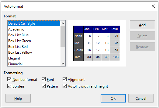
Go to Format > AutoFormat Styles on the Menu bar to open the AutoFormat dialog (Figure 36).
Select the type of format and format color in the list.
Select the formatting properties to be included in the AutoFormat style. Click OK.
Figure 36: AutoFormat dialog
You can define a new AutoFormat so that it becomes available for use in all spreadsheets.
Format the data type, font, font size, cell borders, cell background, and so on for a range of cells.
Select the range, of at least 4x4 cells.
Go to Format > AutoFormat Styles to open the AutoFormat dialog. Click Add.
In the Name box of the Add AutoFormat dialog that opens, type a meaningful name for the new format.
Click OK to save. The new AutoFormat is now available in the Format list on the AutoFormat dialog.
Note
The new AutoFormat is stored in your computer user profile and is not available to other users. However, you can use it in other spreadsheets. Other users can import the new AutoFormat by selecting a common style from a table range in the spreadsheet and defining it as a new AutoFormat.
Calc comes with a predefined set of formatting themes (set of styles) that can be applied to spreadsheets. You cannot add new themes to Calc, but you can modify a theme’s styles after the theme is applied to the spreadsheet. All modified styles are only available for use in that spreadsheet.
To apply a theme to a spreadsheet:
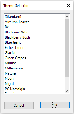
Go to Format > Spreadsheet Theme on the Menu bar or click the Spreadsheet Theme icon on the Tools toolbar to open the Theme Selection dialog (Figure 37).
Select the theme that you want to apply. The theme styles are immediately visible on the underlying spreadsheet.
Click OK.
Figure 37: Theme Selection dialog
Selecting a spreadsheet theme adds several new cell styles to the spreadsheet and modifies the Default cell style.
If you wish, you can now open the Styles deck on the Sidebar to modify specific styles. These changes do not modify the theme; they only change the appearance of the style in the specific spreadsheet you are using. For more about modifying styles, see Chapter 4, Working with Styles, Templates, and Hyperlinks.
Caution
Applying a new theme over an existing one will override all existing theme styles customization with the new theme styles.
Document themes collect various format selections into a set that can be applied and changed quickly. Theme colors were implemented in LibreOffice 7.6; font and format settings are planned for later releases.
Calc supplies several sets of theme colors, and you can define other sets. Theme colors have names like Dark 1, Light 2, Accent 3, and so on. They can be used in styles or applied manually.
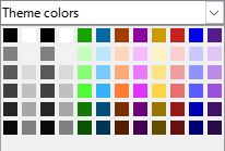
To set up a spreadsheet to use themes, choose colors for fonts, backgrounds, or objects from the Theme colors palette (Figure 38), not an ordinary color palette. The first row of the palette contains the theme colors, with other rows containing modifications. For example, the top-left color in the palette is the currently selected theme’s Dark 1 color; the leftmost color in the second row is a 50% lighter version of Dark 1; the entry at the intersection of the second column and third row is a 15% darker version of Light 1; and so on. You can hover the pointer over any palette cell to see a tooltip indicating the detail of that color.
Figure 38: A palette of theme colors
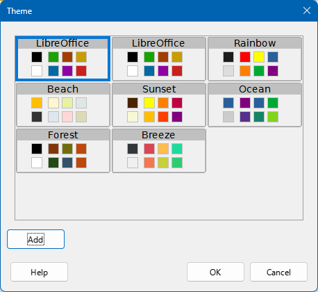
To change the set of theme colors, choose Format > Theme on the Menu bar and select a different theme on the Theme dialog (Figure 39). Colors defined as theme colors change in the document. You need not change any style and need not change any object individually.
Figure 39: Theme dialog
For more information, see Chapter 5, Using Styles and Templates, in the Calc Guide.
Calc can change cell formats depending on user-specified conditions, and those conditions can be imposed in a specified order. For example, a table can show all the values above a specific average in green and all those below that average in red. Conditional formatting also allows you to add graphic icons and data bars to the cell background.
Conditional formatting depends upon the use of styles, and the AutoCalculate feature (Data > Calculate > AutoCalculate) must be enabled. See Chapter 4, Formatting Data, in the Calc Guide for details.
A filter is a tool that hides or displays records within a sheet based on a set of filtering conditions. Similar to sorting, filters are useful for narrowing down long lists of data in order to find particular data items. In Calc, three types of filter exist:
AutoFilter – the most straightforward filter type, providing access to a combo box through arrowhead buttons located at the top of one or more data columns. This box provides options for basic sorting (ascending and descending); sorting by background or font color; filtering by background or font color; filtering by condition (empty, not empty, top 10, and bottom 10); and others.
Standard filter – more complex than AutoFilters, allowing for up to eight filter conditions. Powerful filters can be set up using regular expressions. Also, unlike AutoFilters, standard filters use a dialog to define the conditions.
Advanced filter – filter conditions are stored in a sheet rather than entered into a dialog.
Setting up and using filters are explained in Chapter 2, Entering and Editing Data, in the Calc Guide.
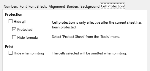
Cells can be password-protected to prevent unauthorized users from making changes. Protected cells can optionally be hidden. Use the Cell Protection tab of the Format Cells dialog (Figure 40) to set up cell protection and toggle the hidden status of protected cells.
Figure 40: Cell Protection tab in Format Cells dialog
Once all desired cells have been flagged with either a protected or unprotected status:
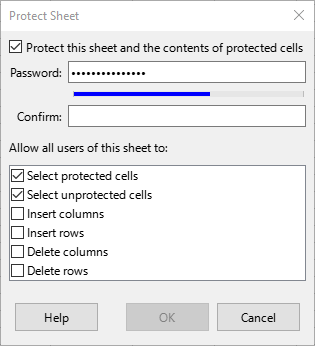
Go to Tools > Protect Sheet, or right-click on the sheet’s tab and select Protect Sheet in the context menu. The Protect Sheet dialog opens (Figure 41).
Select Protect this sheet and the contents of protected cells.
Type a password and then confirm the password. The dialog provides a password strength meter to indicate the strength of the entered password. This incorporates a colored bar to reflect password strength, with red indicating a weak password and green indicating a strong password. In addition, the longer the colored bar, the greater the strength of the password.
Select or deselect the elements to protect from user actions.
Click OK.
Figure 41: Protect Sheet dialog with password strength meter
Any cells that had been marked as protected will no longer be editable by anyone that does not have the password.
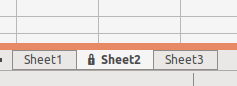
The protected sheet has a padlock icon in its tab, as shown in Figure 42.
Figure 42: The padlock icon in a protected sheet
Alternatively, the entire spreadsheet can be password-protected by selecting Tools > Protect Spreadsheet Structure on the Menu bar. When this option is chosen, unauthorized users cannot add, delete, move, or rename any sheets in the document.
When Calc sorts cells in a sheet, they are re-ordered based on user-specified sort criteria. Sorts are useful when you are searching for a particular item and become even more useful after you have filtered data.
Also, sorting allows you to add new information to the bottom of your spreadsheet and then use a sort to put the values in their proper order. When a spreadsheet is long, it is usually easier to add new information at the bottom of the sheet, rather than adding rows in their correct place. After you have added information, you can then sort the records to update the spreadsheet.
For more information on sorting records and the sorting options available, see Chapter 2, Entering and Editing Data, in the Calc Guide.
To use the Sort dialog on cells in a spreadsheet:
Select the cells to be sorted.
Go to Data > Sort on the Menu bar, or click the Sort icon on the Standard toolbar, to open the Sort dialog (Figure 43).
On the Sort Criteria tab, select the sort criteria in the drop-down lists. The selected lists are populated from the selected cells.
Select either ascending order (A-Z, 0-9) or descending order (Z-A, 9-0).
Adjust the settings as required on the Sort Criteria and Options tabs. For details, see the Help or Chapter 2, Entering and Editing Data, in the Calc Guide.
Click OK and the sort is carried out on the spreadsheet.
Figure 43: Sort dialog, Sort Criteria tab
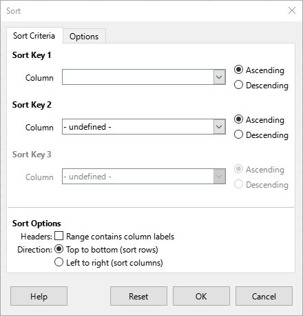
Users can add a comment to a cell. These comments are small notes and text that provide extra information about the spreadsheet. They are not considered a part of the spreadsheet for calculation or printing purposes, and usually only appear when the user hovers the mouse over the particular cell that has been commented.
You can insert a comment by any of the following actions:
Right-clicking on the desired cell and selecting Insert Comment in the context menu.
Selecting Insert > Comment on the Menu bar.
Pressing Ctrl+Alt+C.
Clicking the Insert Comment icon on the Standard toolbar.
Cells that contain comments are marked with a colored triangle in the upper right corner. By default, comments will remain hidden and only appear when you hover the mouse over a cell that contains a comment. To toggle the visibility of comments, select View > Comments on the Menu bar.
For more information, see Chapter 12, Sharing and Reviewing Spreadsheets, in the Calc Guide.
You may need more than numbers and text in a spreadsheet. Often the contents of one cell depend on the contents of other cells. Formulas are equations that use numbers and variables to produce a result. Any cell can contain a formula. Variables are placed in cells to hold data required by equations.
A function is a predefined calculation entered in a cell to help you analyze or manipulate data. All you have to do is enter the arguments and the calculation is made automatically. Functions help you create the formulas required to get the results that you are looking for.
Functions and formulas can be entered directly into the Formula bar or by using the Function Wizard. To launch the Function Wizard, click the Function Wizard icon on the Formula bar, select Insert > Function on the Menu bar, or press Ctrl+F2.
Inside the Function Wizard, you can choose from the many built-in Calc functions available. When you search for a term in the Function Wizard, function descriptions are provided as well as their names. You can also choose to complete functions from within the wizard rather than having to type full formulas into the Formula bar.
Each function, when selected, will display a brief explanation of its use and acceptable syntax. It will also allow you to enter the information required by that function and a result window will showing the expected calculation from the data entered.
Note
A fast alternative to the Function Wizard is the Functions deck on the Sidebar, where you can quickly list and narrow down functions. It provides brief explanations on their use and syntax, but does not provide the search or data entry capabilities of the full wizard.
Calc offers powerful built-in functions under multiple categories, covering Database, Date & Time, Financial, Information, Logical, Mathematical, Array, Statistical, Spreadsheet, Text, and Add-in functions.
For a more in-depth introduction to formulas and the Function Wizard, see Chapter 8, Using Formulas and Functions, in the Calc Guide.
Figure 44: Function Wizard
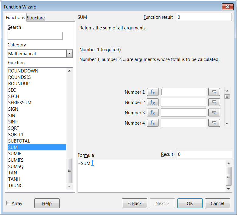
Calc includes many tools to help you analyze information, including features for copying and reusing data, for automatically creating subtotals, and other ways to vary information and help you find the answers you need. These tools are divided between the Tools and Data menus.
Calc also includes many tools for statistical analysis, and they can help you obtain important numerical information on data obtained from physical measurements, polls, or even business transactions such as sales, stock quotations, and so on. These statistical data analyses are available in the menu Data > Statistics.
See Chapter 10, Data Analysis, in the Calc Guide for more information on the these tools.
One of the most useful tools for analyzing data is the pivot table, which allows you to organize, manipulate, and summarize large amounts of data to make it much easier to read and understand. They also allow you to answer different questions about a spreadsheet by rearranging – or pivoting – the data in it, which includes the ability to view different summaries of the source data, display the details of areas of interest, and create reports. You can also create a pivot chart that allows you to view a graphical representation of the data in a pivot table.
For example, you might have a spreadsheet containing a list of donations to various charities by a group of recruiters in various months, but you are only interested in how much money each recruiter has collected in total. Instead of manually calculating that amount by using the sorting and formatting options, you could arrange a pivot table which makes that data easier to organize and read.
To create a pivot table, choose Data > Pivot Table > Insert or Edit on the Menu bar, or click the Insert or Edit Pivot Table icon on the Standard toolbar. The Pivot Table Layout dialog will intelligently guess the column headings from the provided raw data and insert them into the Available Fields selection box. From there, you can drag and drop your desired information into column, row, data, or filter fields to organize accordingly and click OK to view the results.
To choose new information to display, or to alter the layout of the existing information, right-click anywhere in the existing pivot table to bring up the context menu and choose Properties. You can also access the same dialog by selecting Data > Pivot Table > Insert or Edit on the Menu bar, or clicking the Insert or Edit Pivot Table icon on the Standard toolbar.
For an in-depth explanation of pivot tables and the preconditions necessary to use them, see Chapter 9, Using Pivot Tables, in the Calc Guide.
To get a quick visual representation of the data contained in a pivot table, you can generate a pivot chart. Functionally, pivot charts are nearly identical to regular charts except in two key areas. First, as the data in the pivot table is altered, the pivot chart will adjust itself automatically. Second, a pivot chart includes field buttons, which are graphical elements that allow you to filter the content of the pivot table from within its pivot chart.
For more information on pivot charts and charts in general, see Chapter 3, Creating Charts and Graphs, and Chapter 9, Using Pivot Tables, in the Calc Guide.
Printing from Calc is similar to printing from other LibreOffice components (see Chapter 1, LibreOffice Basics), but some details of printing in Calc are different, especially regarding preparation for printing.
After print ranges have been defined, they are formatted with automatic page breaks. To view the page breaks, go to View > Page Break on the Menu bar.
Print ranges can be used to print a specific part of the data and print selected rows or columns on every page. For more information about using print ranges, see Chapter 7, Printing, Exporting, Emailing, and Signing in the Calc Guide.
To define a new print range or modify an existing print range:
Select the range of cells to be included in the print range.
Go to Format > Print Ranges > Define on the Menu bar. Automatic page break lines are displayed on screen.
To check the print range, go to File > Print Preview on the Menu bar, press Ctrl+Shift+O, or click the Toggle Print Preview icon on the Standard toolbar. Calc will display only the cells in the print range.
After defining a print range, you can add more cells to it by creating another print range. This allows multiple, separate areas of the same sheet to be printed while not printing the whole sheet.
After defining a print range, select an extra range of cells for adding to the print range.
Go to Format > Print Ranges > Add on the Menu bar to add the extra cells to the print range. The page break lines are no longer displayed on the screen.
To check the print ranges, go to File > Print Preview on the Menu bar, press Ctrl+Shift+O, or click the Toggle Print Preview icon on the Standard toolbar. Calc will display the print ranges as separate pages.
Note
The additional print range will print as a separate page, even if both ranges are on the same sheet.
It may become necessary to remove a defined print range, for example, if the whole sheet needs to be printed later.
To remove all the defined print ranges, go to Format > Print Ranges > Clear on the Menu bar. After the print ranges have been removed, the default page break lines will appear on the screen.
At any time, you can directly edit the print range, for example to remove or resize part of the print range. Go to Format > Print Ranges > Edit on the Menu bar to open the Edit Print Ranges dialog where you can modify the print range.
To select the options for page order, elements to be printed, and scale to be used when printing a spreadsheet:
Go to Format > Page Style on the Menu bar to open the Page Style dialog (Figure 45).
Select the Sheet tab and make your selections from the available options. Click OK.
Figure 45: Page Style dialog – Sheet tab
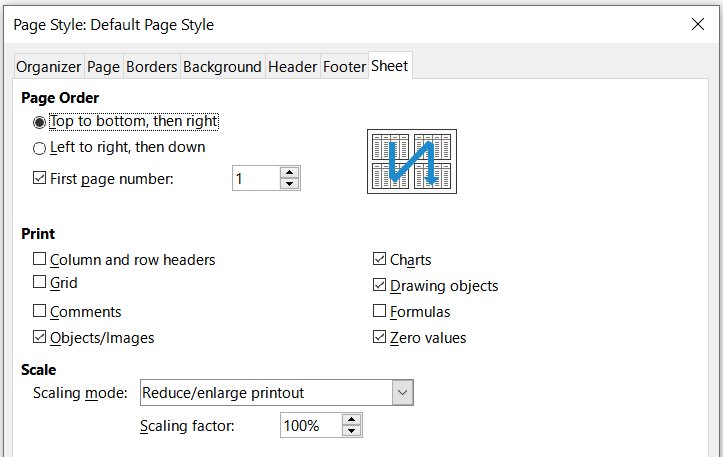
If a sheet is printed on multiple pages, you can set up certain rows or columns to repeat on each printed page. For example, if the top two rows of the sheet as well as column A need to be printed on all pages, do the following:
Go to Format > Print Ranges > Edit on the Menu bar to open the Edit Print Ranges dialog (Figure 46).
Type the row identifiers in the Rows to Repeat box. For example, to repeat rows 1 and 2, type $1:$2. This automatically changes Rows to Repeat from - none - to - user defined -.
Type the column identifiers in the Columns to Repeat box. For example, to repeat column A, type $A. In Columns to Repeat, - none - changes to - user defined -.
Click OK.
For more information on editing print ranges, see Chapter 7, Printing, Exporting, Emailing, and Signing, in the Calc Guide.
Figure 46: Edit Print Ranges dialog
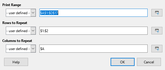
While defining a print range can be a powerful tool, it may sometimes be necessary to manually adjust the printout using a manual page break. A page break helps to ensure that the data prints properly according to the page size and page orientation. You can insert a horizontal page break above or a vertical page break to the left of the active cell.
To insert a page break:
Navigate to the cell where the page break is needed.
Go to Sheet > Insert Page Break on the Menu bar.
Select Row Break to create a horizontal page break above the selected cell or select Column Break to create a vertical page break to the left of the selected cell.
Tip
After selecting View > Page Break, you can right-click on a cell to access a context menu containing Row Break and Column Break options.
To remove a page break:
Navigate to a cell that is next to the page break you want to remove.
Go to Sheet > Delete Page Break on the Menu bar.
Select Row Break or Column Break as needed.
Tip
Multiple manual row and column breaks can exist on the same sheet. When you want to remove them, you can remove each break individually, as described above. However, after selecting View > Page Break, you can right-click on a cell to access a context menu containing a Delete All Breaks option to remove them all at once.
For more information on page breaks, see Chapter 7, Printing, Exporting, Emailing, and Signing, in the Calc Guide.
Headers and footers are text that can be printed at the top or bottom of a page when a you print a spreadsheet. Headers and footers are set and defined using the same method. For more information on setting and defining headers and footers, see Chapter 7, Printing, Exporting, Emailing, and Signing, in the Calc Guide.
Headers and footers are also assigned to a page style. You can define more than one page style for a spreadsheet and assign different page styles to different sheets within a spreadsheet. For more information, see Chapter 5, Using Styles and Templates, in the Calc Guide.
To set a header or footer:
Select the sheet that you want to set the header or footer for.
Open the Page Style dialog (Figure 47) using one of the following methods:
Go to Format > Page Style on the Menu bar.
On the Styles deck of the Sidebar, right-click the relevant page style and select Modify in the context menu.
Double-click the name of the page style on the Status Bar.
Select the Header or Footer tab as appropriate.
Select the Header on or Footer on option.
Select Same content on left and right pages if you want the same header or footer to appear on all the printed pages.
Select / deselect Same content on first page as required.
Set the margins, spacing, and height for the header or footer. You can also select AutoFit height to automatically adjust the height of the header or footer.
To change the appearance of the header or footer, click on More to open the Border / Background dialog.
To set the contents, for example page number, date and so on, that appear in the header or footer, click Edit to open the Headers (or Footers) dialog.
Click OK to save your changes.
Figure 47: Header tab of Page Style dialog