Getting Started Guide 7.3
Chapter 5,
Getting Started with Calc
Using spreadsheets in LibreOffice
This document is Copyright © 2022 by the LibreOffice Documentation Team. Contributors are listed below. You may distribute it and/or modify it under the terms of either the GNU General Public License (http://www.gnu.org/licenses/gpl.html), version 3 or later, or the Creative Commons Attribution License (http://creativecommons.org/licenses/by/4.0/), version 4.0 or later.
All trademarks within this guide belong to their legitimate owners.
To this edition
|
Jean Hollis Weber |
Vasudev Narayanan |
|
|
Vasudev Narayanan |
Felipe Viggiano |
Kees Kriek |
|
Jean Hollis Weber |
Steve Fanning |
Olivier Hallot |
|
Amanda Labby |
Jorge Rodriguez |
Paul Figueiredo |
|
Dave Barton |
|
|
Please direct any comments or suggestions about this document to the Documentation Team’s mailing list: documentation@global.libreoffice.org
Note
Everything you send to a mailing list, including your email address and any other personal information that is written in the message, is publicly archived and cannot be deleted.
Published February 2022. Based on LibreOffice 7.3 Community.
Other versions of LibreOffice may differ in appearance and functionality.
Some keystrokes and menu items are different on macOS from those used in Windows and Linux. The table below gives some common substitutions for the instructions in this book. For a more detailed list, see the application Help.
|
Windows or Linux |
macOS equivalent |
Effect |
|
Tools > Options |
LibreOffice > Preferences |
Access setup options |
|
Right-click |
Control+click and/or right-click depending on computer setup |
Open a context menu |
|
Ctrl (Control) |
⌘ (Command) |
Used with other keys |
|
Alt |
⌥ (Option) or Alt, depending on keyboard |
Used with other keys |
|
F11 |
⌘+T |
Open Styles deck in Sidebar |
Calc is the spreadsheet component of LibreOffice. You can enter data (usually numerical) in a spreadsheet and then manipulate this data to produce certain results.
Alternatively, you can enter data and then use Calc in a “What if...” manner by changing some of the data and observing the results without having to retype the entire spreadsheet or sheet.
Other features provided by Calc include:
Functions, which can be used to create formulas to perform complex calculations on data.
Database functions, to arrange, store, and filter data.
Dynamic charts, including a wide range of 2D and 3D charts.
Macros, for recording and executing repetitive tasks; scripting languages supported include LibreOffice Basic, Python, BeanShell, and JavaScript.
Ability to open, edit, and save Microsoft Excel spreadsheets.
Import and export of spreadsheets in multiple formats, including HTML, CSV (without or with formulas), dBase, PDF, and PostScript.
Collaborate with others seamlessly by sharing the spreadsheet.
Simple wildcards such as the asterisk (*), question mark (?), and tilde (~) from other spreadsheet applications are recognized by LibreOffice in formula expressions.
By default, LibreOffice Calc uses its own formula syntax, referred to as Calc A1, rather than the Excel A1 syntax used by Microsoft Excel. LibreOffice will translate seamlessly between the two. However, if you are familiar with Excel you may wish to change the default syntax in Calc by going to Tools > Options > LibreOffice Calc > Formula and choosing Excel A1 or Excel R1C1 in the Formula syntax drop-down menu.
For more information on formula syntax, see Chapter 7, Using Formulas and Functions, in the Calc Guide.
Microsoft Office uses Visual Basic for Applications (VBA) code, and LibreOffice uses Basic code based on the LibreOffice API. Although the programming languages are the same, the objects and methods are different and therefore not entirely compatible.
LibreOffice can run some Excel Visual Basic scripts if you enable this feature at Tools > Options > Load/Save > VBA Properties.
If you want to use macros written in Microsoft Excel using the VBA macro code in LibreOffice, you must first edit the code in the LibreOffice Basic IDE editor.
For more information, refer to Chapter 12, Calc Macros, in the Calc Guide.
Calc works with documents called spreadsheets. Spreadsheets consist of a number of individual sheets, each sheet containing cells arranged in rows and columns. A particular cell is identified by its row number and column letter.
Cells hold the individual elements – text, numbers, formulas, and so on – that make up the data to display and manipulate.
Each spreadsheet can have up to 10,000 sheets, and each sheet can have a maximum of 1,048,576 rows and a maximum of 1024 columns.
When Calc is started, the main window opens (Figure 1). The parts of this window are described below. You can show or hide many of the parts as desired, using the View menu on the Menu bar.
Figure 1: Calc main window
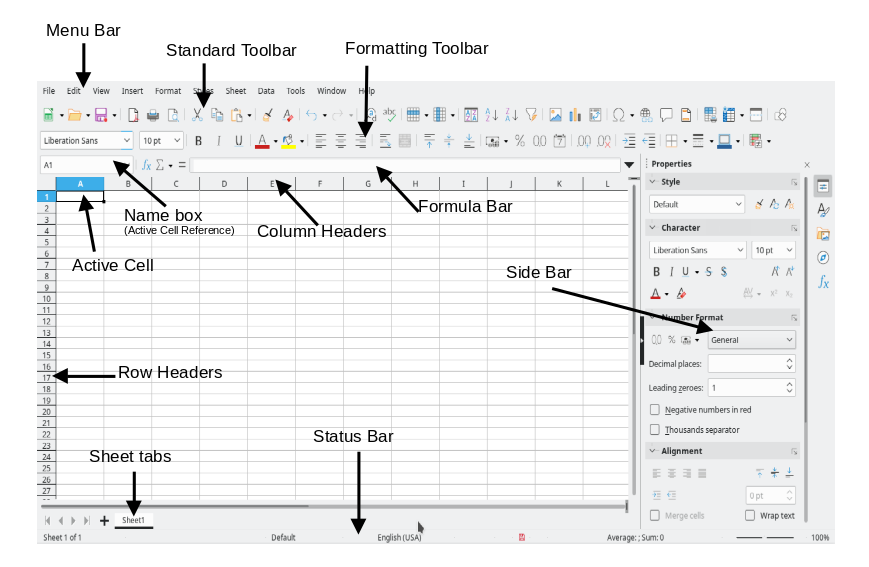
The Title bar, located at the top, shows the name of the current spreadsheet. When a spreadsheet is newly created from a template or a blank document, its name is Untitled X, where X is a number. When you save a spreadsheet for the first time, you are prompted to enter a name of your choice.
Under the Title bar is the Menu bar. When you select one of the menu items, a sub-menu drops down to show commands. You can also customize the Menu bar; see Chapter 14, Customizing LibreOffice, for more information.
Most of the menus are similar to those in other components of LibreOffice, although the specific commands and tools may vary. The menus specific to Calc are Sheet and Data; in addition, several important data analysis tools are found in the Tools menu.
Sheet
Data
Tools
View
In a default LibreOffice installation, the top docked toolbar, just under the Menu bar, is called the Standard toolbar. It is consistent across the LibreOffice applications. The position and use of it and other toolbars are described in Chapter 1, Introducing LibreOffice.
The Formula Bar (Figure 2) is located at the top of the sheet in the Calc workspace. It is permanently docked in this position and cannot be used as a floating toolbar. However, it can be hidden or made visible by selecting or deselecting View > Formula Bar on the Menu bar.
Figure 2: Formula Bar

From left to right, the Formula Bar includes the following:
Figure 3: Select Function drop-down
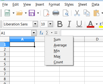
You can also directly edit the contents of a cell by double-clicking on the cell. When you enter or edit data in a cell, the Select Function and Formula icons change to Cancel and Accept icons.
Note
In a spreadsheet, the term “function” covers much more than just mathematical functions. See Chapter 7, Using Formulas and Functions, in the Calc Guide for more information.
The Calc Status bar (Figure 4 and Figure 5) provides information about the spreadsheet as well as quick and convenient ways to change some of its features. Most of the fields are similar to those in other components of LibreOffice. See Chapter 1, Introducing LibreOffice, for more information.
Figure 4: Calc Status bar (left)
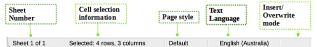
Figure 5: Calc Status bar (right)
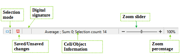
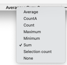
The Status bar has a quick way to do some math operations on selected cells in the spreadsheet. You can view the calculated average and sum, count of elements, and more on the selection by right-clicking over the Cell/Object Information area and selecting the operations you want to display in the Status bar (Figure 6).
Figure 6: Selecting math operations to show on Status bar
The Calc Sidebar (View > Sidebar or Ctrl+F5) is located on the right side of the window. It is a mixture of toolbar and dialog. It is similar to the Sidebar in Writer (shown in Chapter 1 and Chapter 4 of this book) and consists of five decks: Properties, Styles, Gallery, Navigator, and Functions. Each deck has a corresponding icon on the Tab panel to the right of the sidebar, allowing you to switch between them. The decks are described below.
Properties
Styles, Gallery, Navigator
Functions
The main section of the workspace in Calc displays the cells in the form of a grid. Each cell is formed by the intersection of one column and one row in the spreadsheet.
At the top of the columns and the left of the rows are a series of header boxes containing letters and numbers. The column headers use an alpha character starting at A and go on to the right. The row headers use a numerical character starting at 1 and go down.
These column and row headers form the cell references that appear in the Name Box on the Formula Bar (Figure 2). If the headers are not visible on the spreadsheet, choose View > View Headers on the Menu bar.
Each Calc spreadsheet can contain multiple sheets. At the bottom of the grid of cells are sheet tabs indicating how many sheets are in the spreadsheet. By default, a new spreadsheet is created with one sheet named Sheet1. Click on a tab to display that sheet. An active sheet is indicated with a white tab (default Calc setup). You can also select multiple sheets by holding down the Ctrl key while clicking on the sheet tabs.
To change the default name for a sheet (Sheet1, Sheet2, and so on), right-click on a sheet tab and select Rename Sheet in the context menu, or double-click on the sheet tab, to open the Rename Sheet dialog where you can type a new name for the sheet.
To change the color of a sheet tab, right-click on the tab and select Tab Color in the context menu to open the Tab Color dialog. Select a color and click OK. To add new colors to this color palette, see Chapter 14, Customizing LibreOffice.
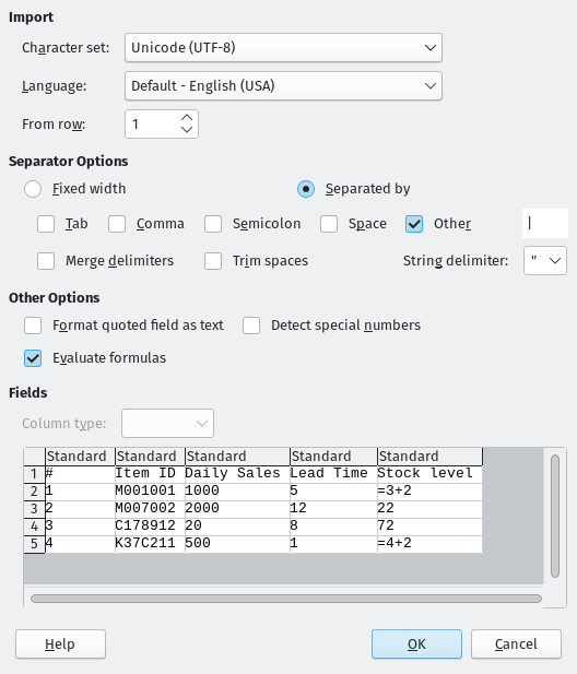
Comma-separated values (CSV) files are spreadsheet files in a text format where cell contents are separated by a character, for example a comma or semicolon or any other character like vertical bar. Each line in a CSV text file represents a row in a spreadsheet. Text is entered between quotation marks; numbers are entered without quotation marks. It treats data as a formula if the column value begins with an equal sign (=).
Figure 7: Text Import dialog
Note
Most CSV files come from database tables, queries, or reports, where further calculations and charting are required.
1) Choose File > Open on the Menu bar and locate the CSV file. Most CSV files have the extension .csv. However, some CSV files may have a .txt extension.
2) Select the file and click Open.
3) On the Text Import dialog (Figure 7), select the required options for importing the CSV file into the Calc spreadsheet. For details about these options, see Chapter 1, Introducing Calc, in the Calc Guide.
4) Click OK to import the file.
For information on how to save files manually or automatically, see Chapter 1, Introducing LibreOffice. Calc can save spreadsheets in a range of formats and also export spreadsheets to PDF, HTML, XHTML file formats and JPEG and PNG images formats; see Chapter 6, Printing, Exporting, E-mailing, and Signing, in the Calc Guide for more information.
You can save a spreadsheet in another format:
1) Save the spreadsheet in Calc spreadsheet file format (*.ods).
2) Select File > Save As on the Menu bar to open the Save As dialog.
3) In the File name field, you can enter a new file name for the spreadsheet.
4) In the File type drop-down list, select the type of spreadsheet format you want to use.
5) If Automatic file name extension is present and selected, the correct file extension for the spreadsheet format you have selected will be added to the file name.
6) Click Save.
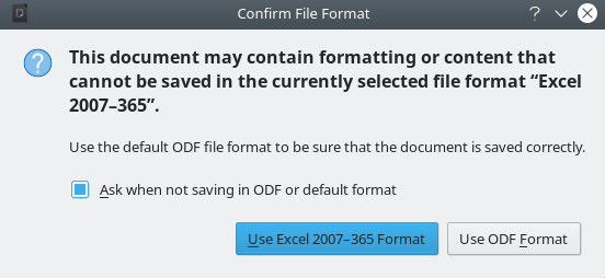
When a spreadsheet file is saved in a format other than .ods, the Confirm File Format dialog opens (Figure 8). Click Use [xxx] Format to continue saving in your selected spreadsheet format or click Use ODF Format to save the spreadsheet in Calc .ods format. If you uncheck Ask when saving in ODF or default format, this dialog no longer appears when saving in another format.
Figure 8: Confirm File Format dialog
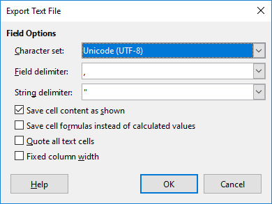
If you select Text CSV format (*.csv) for your spreadsheet, the Export Text File dialog (Figure 9) opens. Here you can select the character set, field delimiter, string (text) delimiter, and so on to be used for the CSV file.
Figure 9: Export Text File dialog for CSV files
Note
Once you have saved a spreadsheet in another format, all changes you make to the spreadsheet will now occur only in the format you are using. If you want to go back to working with a *.ods version, you must save the file as a *.ods file.
Tip
To have Calc save spreadsheets by default in a file format other than .ods, go to Tools > Options > Load/Save > General. In the Default File Format and ODF Settings area, select Spreadsheet in Document type, then in Always save as, select your preferred file format.
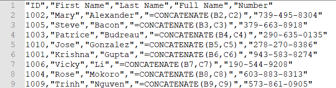
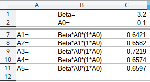
Calc can export raw data and calculated data as a CSV file. An example of data for export is shown in Figure 10, and the resulting CSV file is shown in Figure 11.
The steps to export are:
1) Click the sheet to be written as a CSV file.
2) Choose Tools > Options > LibreOffice Calc > View on the Menu bar.
3) Under Display, mark the Formulas check box. Click OK.
4) Choose File > Save as.
5) On the Save as dialog, select Text CSV in the File type field.
6) Enter a filename and click Save.
7) From the Export of text files dialog that appears, select the character set and the field and text delimiters for the data to be exported, and confirm with OK.
Figure 10: Exporting raw and calculated values
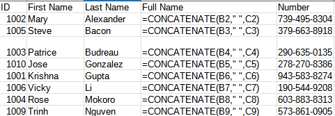
Figure 11: CSV file containing raw and calculated values
To send a fragment of a spreadsheet to someone or publish it on the Internet, you can export a range selection or a selected group of shapes (images) to a PNG or JPG graphics format:
1) Select the cell range or the group of shapes, then select File > Export.
2) In the Export dialog, type a name for the image, select the graphics file format, and mark the Selection checkbox.
3) Click Export or Save, as appropriate.
Calc may open a further dialog for you to configure the settings associated with the selected graphics format.
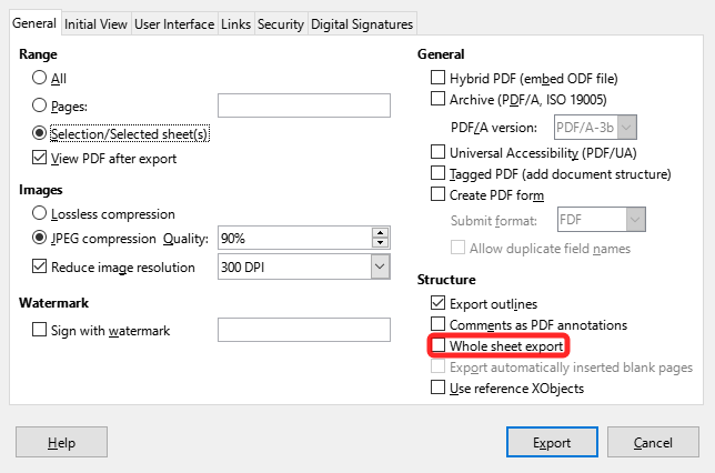
Calc can export the entire contents of a sheet as a PDF in one page. It is easier to preview the contents on one page to understand if it requires any changes.
The steps to export the contents to one page:
1) From the Menu bar, select File > Export as PDF.
2) On the General tab of the PDF options dialog (Figure 12), select the option Whole sheet export.
3) Click the Export button, and choose a location for the PDF.
Figure 12: Exporting sheets to PDF as one page
Calc can import data using web query by linking to an external data source. You can filter or choose the table to import by HTML caption:
1) Position the cursor in the cell where you want the new content to be imported.
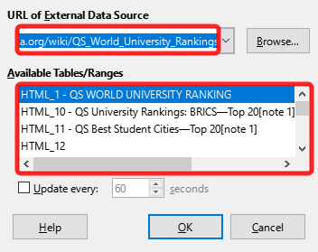
2) Choose Sheet > Link to External Data to open the External Data dialog (Figure 13).
3) Enter the URL of the HTML document or the name of the spreadsheet, then press Enter. You can also click the Browse button to open a file selection dialog.
4) In the Available Tables/Ranges list box, select the named ranges or tables you want to insert. You can also specify that the ranges or tables are updated every n seconds. These tables are now listed in the order they appear in the source.
5) Click OK to finish.
Figure 13: Link to external data
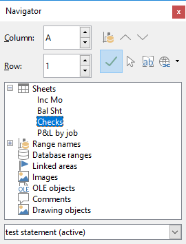
Calc provides many ways to navigate within a spreadsheet from cell to cell and sheet to sheet. You can generally use the method you prefer.
When a cell is selected or in focus, the cell borders are emphasized. When a group of cells is selected, the cell area is colored. The color of the cell border emphasis and the color of a group of selected cells depends on the operating system being used and how you have set up LibreOffice.
Figure 14: Calc Navigator
Home moves the cell focus to the start of a row.
End moves the cell focus to the last cell on the right in the row in the right-most column that contains data.
Page Down moves the cell focus down one complete screen display.
Page Up moves the cell focus up one complete screen display.
Each sheet in a spreadsheet is independent of the other sheets, though references can be linked from one sheet to another. To navigate between sheets in a spreadsheet:
If your spreadsheet contains a lot of sheets, then some of the sheet tabs may be hidden. If this is the case:
Using the four buttons to the left of the sheet tabs can move the tabs into view (Figure 15).
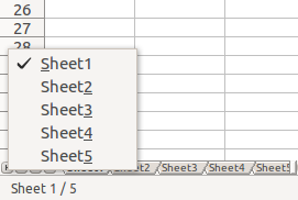
Right-clicking on any of the arrows, or the +, opens a context menu where you can select a sheet (Figure 16).
Figure 15: Navigating sheet tabs
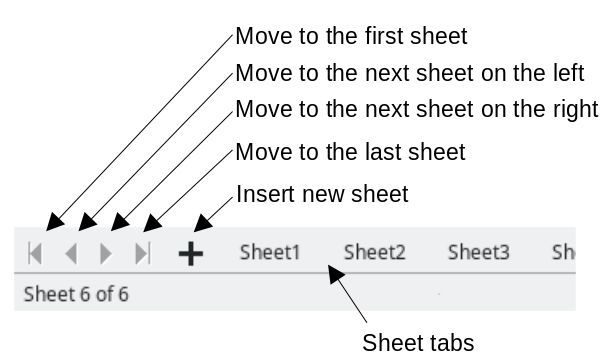
Figure 16: Right-click any active arrow button
Note
When you insert a new sheet into a spreadsheet, Calc automatically uses the next number in the numeric sequence as a name. Depending on which sheet is open when you insert a new sheet, the new sheet may not be in its correct numerical position. It is recommended to rename sheets in a spreadsheet to make them more recognizable.
You can navigate a spreadsheet using the keyboard, by pressing a key or a combination of keys. See Chapter 1, Introduction, and Appendix A, Keyboard Shortcuts, in the Calc Guide for the keys and key combinations you can use for spreadsheet navigation in Calc.
You can choose the direction in which the Enter key moves the cell focus by going to Tools > Options > LibreOffice Calc > General. Use the first two options under Input Settings (Figure 17) to change the Enter key settings.
Figure 17: Customizing the Enter key
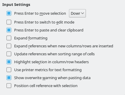
Select the direction cell focus moves from the drop-down list. The Enter key can also be used to switch into and out of editing mode. You can enable or disable the use of Enter to paste the content of a cell that has been copied to the clipboard.
Click in the cell. You can verify your selection by looking in the Name Box on the Formula Bar (Figure 2 above).
A range of cells can be selected using the keyboard or the mouse.
To select a range of cells by dragging the mouse cursor:
1) Click in a cell.
2) Press and hold down the left mouse button.
3) Move the mouse to highlight the desired block of cells, then release the mouse button.
To select a range of cells without dragging the mouse:
1) Click in the cell that is to be one corner of the range of cells.
2) Hold down the Shift key and click in the opposite corner cell of the block of cells.
Tip
You can also select a contiguous range of cells by first clicking in the Selection mode field on the Status bar (Figure 5 above) and selecting Extending selection before clicking in the opposite corner of the range of cells. Make sure to change back to Standard selection or you may extend a cell selection unintentionally.
To select a range of cells without using the mouse:
1) Select the cell that will be one of the corners in the range of cells.
2) While holding down the Shift key, use the cursor arrows to select the rest of the range.
Tip
You can also directly select a range of cells using the Name Box. Click in the Name Box on the Formula Bar (Figure 2 above). Enter the cell reference for the upper left-hand cell, followed by a colon (:), and then the lower right-hand cell reference. For example, to select the range that would go from A3 to C6, you would enter A3:C6.
1) Select the cell or range of cells using one of the methods above.
2) Move the mouse pointer to the start of the next range or single cell.
3) Hold down the Ctrl key and click or click-and-drag to select another range of cells to add to the first range.
4) Repeat as necessary.
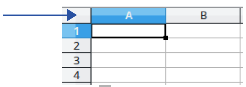
To select a single column, click on the column header (Figure 1 above). To select a single row, click on the row header.
To select multiple columns or rows that are contiguous:
1) Click on the first column or row in the group.
2) Hold down the Shift key.
3) Click the last column or row in the group.
To select multiple columns or rows that are not contiguous:
1) Click on the first column or row in the group.
2) Hold down the Ctrl key.
3) Click on all of the subsequent columns or rows while holding down the Ctrl key.
To select the entire sheet, click on the corner box between the column header A and the row header 1 (Figure 18), or use the key combination Ctrl+Shift+Space to select the entire sheet, or use Edit > Select All on the Menu bar.
Figure 18: Select All box
You can select one or multiple sheets in Calc. It can be advantageous to select multiple sheets, especially when you want to make changes to many sheets at once.
Click on the sheet tab for the sheet you want to select. The tab for the selected sheet becomes white (default Calc setup).
To select multiple contiguous sheets:
1) Click on the sheet tab for the first desired sheet.
2) Hold down the Shift key and click on the sheet tab for the last desired sheet.
3) All tabs between these two selections will turn white (default Calc setup). Any actions that you perform will now affect all the highlighted sheets.
Multiple non-contiguous sheets
To select multiple non-contiguous sheets:
1) Click on the sheet tab for the first desired sheet.
2) Hold down the Ctrl key and click on the sheet tab for the each additional desired sheet.
3) The selected tabs will turn white (default Calc setup).
Right-click a sheet tab and choose Select All Sheets in the context menu, or select Edit > Select > Select All Sheets on the Menu bar.
Using the Sheet menu:
1) Select a cell, column, or row where you want the new column or row inserted.
2) Go to Sheet on the Menu bar and select either Insert Columns > Columns Before, or Insert Columns > Columns After, or Insert Rows > Rows Above, or Insert Rows > Rows Below.
Using the mouse:
1) Select a column or row where you want the new column or row inserted.
2) Right-click the column or row header.
3) Select Insert Columns Before, Insert Columns After, Insert Rows Above, or Insert Rows Below in the context menu.
Multiple columns or rows can be inserted at once rather than inserting them one at a time.
1) Highlight the required number of columns or rows by holding down the left mouse button on the first one and then dragging across the required number of identifiers.
2) Proceed as for inserting a single column or row above.
To hide columns or rows:
1) Select the row or column you want to hide.
2) Go to Format on the Menu bar and select Rows or Columns.
3) Select Hide in the submenu. Alternatively, right-click on the row or column header and select Hide Rows or Hide Columns in the context menu.
To show hidden columns or rows:
1) Select the rows or columns on each side of the hidden row or column.
2) Go to Format on the Menu bar and select Rows or Columns.
3) Select Show in the submenu. Alternatively, right-click on a row or column header and select Show Rows or Show Columns in the context menu.
1) Select the columns or rows you want to delete.
2) Go to Sheet on the Menu bar and select Delete Rows or Delete Columns, or right-click on the column or row header and select Delete Columns or Delete Rows in the context menu.
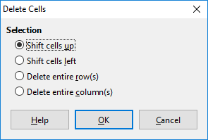
1) Select the cells you want to delete.
2) Go to Sheet > Delete Cells, or press Ctrl+-. Or, right-click on a cell and select Delete in the context menu.
3) Select the option you require from the Delete Cells dialog (Figure 19) and click OK.
Figure 19: Delete Cells dialog
Click on the Add Sheet (+) icon next to the sheet tabs to insert a new sheet after the last sheet in the spreadsheet without opening the Insert Sheet dialog.
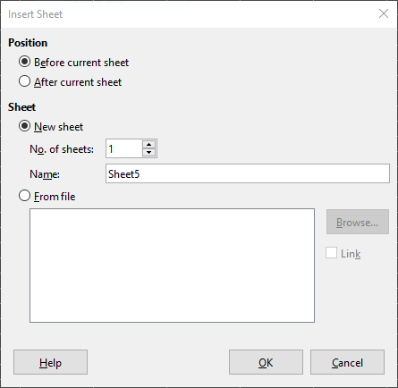
The following methods open the Insert Sheet dialog (Figure 20), where you can position the new sheet, create more than one sheet, name the new sheet, or select a sheet from a file.
Select the sheet where you want to insert a new sheet, then go to Sheet > Insert Sheet on the Menu bar.
Right-click on the sheet tab where you want to insert a new sheet and select Insert Sheet in the context menu.
Click in the empty space at the end of the sheet tabs.
Right-click in the empty space at the end of the sheet tabs and select Insert Sheet in the context menu.
Figure 20: Insert Sheet dialog
You can move or copy sheets within the same spreadsheet by dragging and dropping, or by using the Move/Copy Sheet dialog. To move or copy a sheet into a different spreadsheet, you have to use the Move/Copy Sheet dialog.
In the Move/Copy Sheet dialog (Figure 21), you can specify exactly whether you want the sheet in the same or a different spreadsheet, its position within the spreadsheet, and the sheet name when you move or copy it.
1) In the current document, right-click on the sheet tab you wish to move or copy and select Move or Copy Sheet in the context menu, or go to Sheet > Move or Copy Sheet on the Menu bar.
2) In the Action area, select Move to move the sheet or Copy to copy the sheet.
Figure 21: Move/Copy Sheet dialog
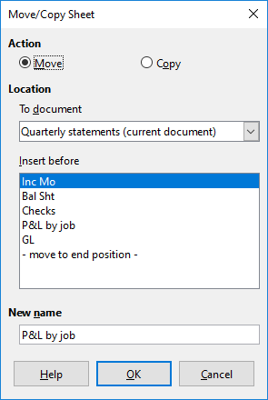
3) Select the spreadsheet where you want the sheet to be placed in the drop-down list in To document. This can be the same spreadsheet, another spreadsheet already open, or a new spreadsheet.
4) Select the position in Insert before where you want to place the sheet.
5) Type a name in the New name box if you want to rename the sheet when it is moved or copied. If you do not enter a name, Calc creates a default name (Sheet2, Sheet3, ...).
6) Click OK to confirm the move or copy and close the dialog.
Caution
When you move or copy to another spreadsheet or a new spreadsheet, a conflict may occur with formulas linked to other sheets in the previous location.
Sometimes you may want to hide the contents of a sheet to preserve data from accidental editing or because its contents are not important to display.
To hide a sheet or many sheets, select the sheet or sheets as above, right-click to open the context menu, and select Hide Sheet.
To show hidden sheets, right-click any sheet tab and select Show Sheet in the context menu. A dialog will open with all hidden sheets listed. Select the desired sheets and then click OK. It is not possible to hide the last visible sheet.
For more information on how to hide and show data, including how to use outline groups and filtering, see Chapter 2, Entering, Editing, and Formatting Data, in the Calc Guide.
Note
Hidden elements are neither visible on a computer display nor printed when a spreadsheet is printed. However, they can still be selected for copying if you select the elements around them. For example, if column B is hidden, it is copied when you select columns A to C. When you require a hidden element again, you can reverse the process and show the element.
By default, the name for each new sheet added is SheetX, where X is the sequential number of the next sheet to be added. While this works for a small spreadsheet with only a few sheets, it can become difficult to identify each one when a spreadsheet contains many sheets.
To rename a sheet, use one of these methods:
Enter the name in the Name text box when you create the sheet using the Insert Sheet dialog (Figure 20 above).
Right-click on a sheet tab and select Rename Sheet in the context menu to replace the existing name with a different one.
Double-click on a sheet tab to open the Rename Sheet dialog.
Note
Sheet names must start with either a letter or a number; other characters, including spaces, are not allowed. Apart from the first character of the sheet name, permitted characters are letters, numbers, spaces, and the underscore character. Attempting to rename a sheet with an invalid name will produce an error message.
To delete a single sheet, right-click on the sheet tab you want to delete and select Delete Sheet in the context menu, or go to Sheet > Delete Sheet on the Menu bar. Click Yes to confirm the deletion.
To delete multiple sheets, select the sheets (see “Selecting sheets” above), then right-click on one of the sheet tabs and select Delete Sheet in the context menu, or go to Sheet > Delete Sheet on the Menu bar. Click Yes to confirm the deletion.
Use the zoom function (View > Zoom) to show more or fewer cells in the window when you are working on a spreadsheet. For more about zoom, see Chapter 1, Introducing LibreOffice.
Freezing is used to lock rows across the top of a spreadsheet or to lock columns on the left of a spreadsheet. Then, when moving around within a sheet, the cells in frozen rows and columns remain in view.
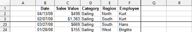
Figure 22 shows some frozen rows and columns. The heavier horizontal line between rows 3 and 23 and the heavier vertical line between columns F and Q indicate that rows 1 to 3 and columns A to F are frozen. The rows between 3 and 23 and the columns between F and Q have been scrolled off the page.
Figure 22: Frozen rows and columns
Often the first row and column contain headings, which you may wish to be visible when scrolling through a long or wide spreadsheet. To quickly freeze either or both of these, use the Freeze Rows and Columns icon on the Standard toolbar for both, or the commands in the drop-down menu of the Freeze Rows and Columns icon: Freeze First Row and Freeze First Column for one of them.
To freeze either rows or columns (single or multiple):
1) Click on the row header below the rows you want the freeze or click on the column header to the right of the columns where you want the freeze.
2) Right-click and choose Freeze Rows and Columns in the context menu, or choose View > Freeze Rows and Columns on the Menu bar, or click the Freeze Rows and Columns icon on the Standard toolbar.
To freeze both rows and columns (single or multiple):
1) Click in the cell that is immediately below the rows you want to freeze and immediately to the right of the columns you want frozen.
2) Choose View > Freeze Rows and Columns on the Menu bar, or click the Freeze Rows and Columns icon on the Standard toolbar.
To unfreeze rows or columns, either use View > Freeze Rows and Columns on the Menu bar, or click on the Freeze Rows and Columns icon on the Standard toolbar. The heavier lines indicating freezing will disappear.
Another way to change the view is by splitting the screen your spreadsheet is displayed in (also known as splitting the window). The screen can be split horizontally, vertically, or both, giving you up to four portions of the spreadsheet in view at one time. An example of splitting the screen is shown in Figure 23, where a split is indicated by additional window borders within the sheet.
This could be useful, for example, when a large spreadsheet has one cell containing a number that is used by three formulas in other cells. By splitting the screen, you can position the cell containing the number in one section of the view and the cells with formulas in other sections. This makes it easy to see how changing the number in one cell affects each of the formulas.
Figure 23: Split screen example
There are two ways to split a screen horizontally or vertically.
Method 1
To split either horizontally or vertically:
1) Click on the row header below the rows where you want to split the screen horizontally or click on the column header to the right of the columns where you want to split the screen vertically.
2) Right-click and choose Split Window in the context menu, or choose View > Split Window on the Menu bar. Window borders appear between the rows or columns indicating where the split has been placed, as shown in Figure 23.
To split both horizontally and vertically at the same time:
1) Click in the cell that is immediately below the rows where you want to split the screen horizontally and immediately to the right of the columns where you want to split the screen vertically.
2) Choose View > Split Window on the Menu bar.
Method 2
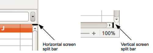
For a horizontal split, click on the thick black line at the top of the vertical scroll bar (Figure 24) and drag the split line below the row where you want the horizontal split positioned.
Similarly, for a vertical split, click on the thick black line at the right of the horizontal scroll bar and drag the split line to the right of the column where you want the vertical split positioned.
Figure 24. Split screen bars
To remove a split view, do one of the following:
Double-click on each split line.
Click and drag the split lines back to their default positions at the ends of the scroll bars.
Go to View on the Menu bar and deselect Split Window.
Right-click on a column or row heading and deselect Split Window in the context menu.
Most data entry in Calc can be done using the keyboard.
Click in the cell and type the number using the number keys on either the main keyboard or the numeric keypad. By default, numbers are right-aligned in a cell.
To enter a negative number, either type a minus (–) sign in front of the number or enclose the number in parentheses, for example (1234). The result for both methods of entry will be the same; in this example, –1234.
If a number is entered with leading zeroes, for example 01481, by default Calc will drop the leading zero. To retain a minimum number of characters in a cell when entering numbers and retain the number format, for example 1234 and 0012, use one of these methods to add leading zeroes.
Method 1
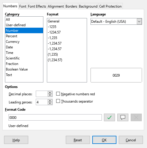
1) With the cell selected, right-click on the cell, select Format Cells in the context menu, or go to Format > Cells on the Menu bar, or use the keyboard shortcut Ctrl+1, to open the Format Cells dialog (Figure 25). Make sure the Numbers tab is selected, then select Number in the Category list.
2) In the Leading zeroes field within the Options area, enter the minimum number of characters required. For example, for four characters, enter 4. Any number less than four characters will have leading zeroes added, for example 12 becomes 0012.
3) Click OK. The number entered retains its number format and any formula used in the spreadsheet will treat the entry as a number in formula functions.
Figure 25: Format Cells dialog – Numbers tab
Method 2
1) Select the cell.
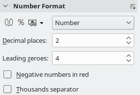
2) On the Sidebar, go to the Properties deck.
3) In the Number Format panel (Figure 26), select Number in the drop-down list, and enter 4 in the Leading zeroes box. Formatting is applied immediately.
Figure 26: Set leading zeroes in Sidebar
Tip
To format numbers with only decimal places, but without a leading zero (for example, .019 instead of 0.019), type a . (period or full stop) followed by ? (question mark) in the Format code box (Figure 25), to represent the number of decimal places required. For example, for 3 decimal places, type .??? and click OK. Any number with only decimal places will then have no leading zero.
Tip
If numerical characters do not need to be treated as numbers in calculations (for example when entering zip codes), you can type an apostrophe (') before the number, for example '01481. When you move the cell focus, the apostrophe is removed, the leading zeroes are retained, and the number is converted to left-aligned text.
Numbers can also be entered as text using one of the following methods.
Method 1
1) With the cell selected, right-click on the cell and select Format Cells in the context menu, or go to Format > Cells on the Menu bar, or use the keyboard shortcut Ctrl+1, to open the Format Cells dialog (Figure 25).
2) Make sure the Numbers tab is selected, then select Text in the Category list.
3) Click OK. The number is converted to text and, by default, left-aligned.
Method 2
1) Select the cell.
2) On the Sidebar, go to the Properties deck. If necessary, click the Open Panel icon (+ or arrow) by Number Format to open that panel (Figure 26).
3) Select Text in the category drop-down list. Formatting is applied to the cell immediately.
Note
By default, any numbers that have been formatted as text in a spreadsheet will be treated as a zero by any formulas used in the spreadsheet. Formula functions will ignore text entries. You can change this feature in Tools > Options > LibreOffice Calc > Formula. In Detailed Calculation Settings, select Custom (conversion of text to numbers and more). Click the Details button, and then select the proper treatment in the Detailed Calculation Settings dialog.
Click in the cell and type the text. By default, text is left-aligned in a cell. Cells can contain several lines of text. If you want to use paragraphs, press Ctrl+Enter to create another paragraph.
On the Formula bar, you can extend the Input line if you are entering several lines of text. Click on the Expand Formula Bar icon located on the right-hand end of the Formula bar and the Input line becomes multi-line.
Select the cell and type the date or time. You can separate the date elements with a slash (/) or a hyphen (–), or use text, for example 10 Oct 2020. The date format automatically changes to the selected format used by Calc.
When entering a time, separate time elements with colons, for example 10:43:45. The time format automatically changes to the selected format used by Calc.
To change the date or time format used by Calc:
1) With the cell selected, open the Format Cells dialog (Figure 25).
2) Make sure the Numbers tab is selected, then select Date or Time in the Category list.
3) Select the date or time format you want to use in the Format list. Click OK.
You can insert a field linked to the date, sheet name, or document name in a cell.
1) Select a cell and double-click to activate edit mode.
2) Right-click and select Insert Field > Date, or Sheet Name, or Document Title in the context menu.
Above those three options are other Date and Time buttons, which will insert the same information but it will not be updated or recalculated as the options mentioned above.
Note
The Insert Field > Document Title command inserts the name of the spreadsheet and not the title defined in the Description tab in the Properties dialog for the file.
Tip
The fields are refreshed when the spreadsheet is saved or recalculated when using the Ctrl+Shift+F9 shortcut.
Calc automatically applies many changes during data input using AutoCorrect, unless you have deactivated any AutoCorrect changes. You can also undo any AutoCorrect changes by using Edit > Undo on the Menu bar, pressing the keyboard shortcut Ctrl+Z, or manually by going back to the change and replacing the AutoCorrection with what you want to actually see.
To change the AutoCorrect options, go to Tools > AutoCorrect Options on the Menu bar to open the AutoCorrect dialog (Figure 27).
Figure 27: AutoCorrect dialog
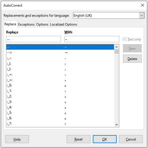
Some AutoCorrect settings are applied when you press the space bar after you enter data. To turn off or on Calc AutoCorrect, go to Tools on the Menu bar and deselect or select AutoInput. See also “AutoInput tool” below.
Entering data into a spreadsheet can be very labor-intensive, but Calc provides several tools for removing some of the drudgery from input.
The most basic ability is to drag and drop the contents of one cell to another with a mouse. Many people also find AutoInput helpful. Calc also includes several other tools for automating input, especially of repetitive material. They include the Fill tool, selection lists, and the ability to input information into multiple sheets of the same document.
The AutoInput tool in Calc automatically completes entries, based on other entries in the same column. When text is highlighted in a cell, AutoInput can be used as follows:
1) To accept the completion, press Enter or F2, or click the left mouse button.
2) To view more completions that start with the same characters, use the key combinations Ctrl+Tab to scroll forward, or Ctrl+Shift+Tab to scroll backward.
3) To see a list of all available AutoInput text items for the current column, use the keyboard combination Alt+Down Arrow.
When typing formulas using characters that match previous entries, a Help tip will appear listing the available functions that start with matching characters. AutoInput ignores the case sensitivity of any data you enter.
By default, AutoInput is activated in Calc. To turn it off, go to Tools on the Menu bar and deselect AutoInput.
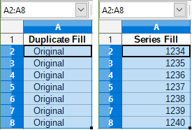
You can use the Fill tool to duplicate existing content or create a series in a range of cells (Figure 28).
1) Select the cell containing the contents you want to copy or start the series from.
2) Drag the cursor in any direction or hold down the Shift key and click in the last cell you want to fill.
3) Go to Sheet > Fill Cells on the Menu bar and select the direction in which you want to copy or create data (Fill Up, Fill Down, Fill Left, or Fill Right), or Fill Series, or Fill Random Number in the submenu.
Tip
You can use the keyboard shortcut Ctrl+D as an alternative to selecting Sheet > Fill Cells > Fill Down on the Menu bar.
Figure 28: Using the Fill tool
Alternatively, you can use a shortcut to fill cells.
1) Select the cell containing the contents you want to copy or start the series from.
2) Move the cursor over the small square in the bottom right corner of the selected cell. The cursor will change shape.
3) Click and drag in the direction you want the cells to be filled. If the original cell contained text, then the text will automatically be copied. If the original cell contained a number, a series will be created.
Caution
When you are selecting cells so you can use the Fill tool, make sure that none of the cells contain data, except for the cell data you want to use. When you use the Fill tool, any data contained in the selected target cells is overwritten.
When you select a series fill from Sheet > Fill Cells > Fill Series, the Fill Series dialog (Figure 29) opens. Here you can select the type of series you want.
Figure 29: Fill Series dialog
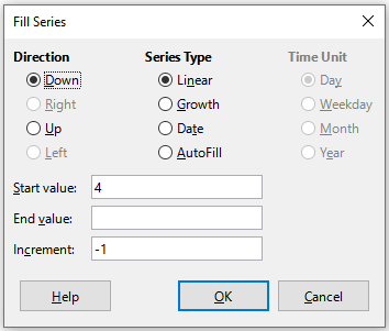
If you select the AutoFill option on the Fill Series dialog, type some text in the Start value field, and press OK, Calc will check if one of your predefined sort lists contains that text. If there is a sort list containing that text, Calc uses the entries in that sort list to fill cells. Go to Tools > Options > LibreOffice Calc > Sort Lists to view your currently defined sort lists.
To define your own sort list, which can later be used as a fill series:
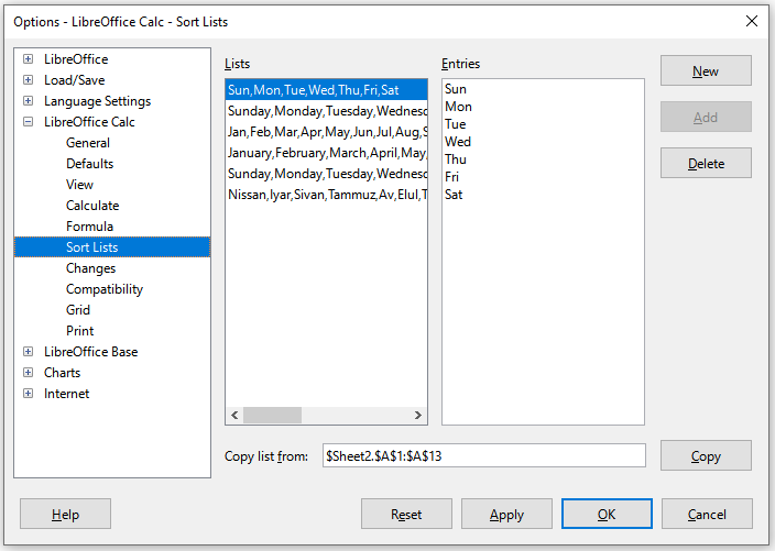
1) Go to Tools > Options > LibreOffice Calc > Sort Lists to open the Sort Lists dialog (Figure 30). This dialog shows the previously-defined series in the Lists box and the contents of the highlighted list in the Entries box.
2) Click New and the Entries box is cleared.
3) Type the series for the new list in the Entries box (one entry per line).
4) Click Add and the new list will now appear in the Lists box.
5) Click OK to save the new list.
Selection lists are available only for text and are limited to using only text that has already been entered in the same column.
1) Select a blank cell in a column that contains cells with text entries.
2) Right-click and select Selection Lists in the context menu, or press Alt+Down Arrow. A drop-down list appears listing any cell in the same column that either has at least one text character or whose format is defined as text.
3) Click on the text entry you require and it is entered into the selected cell.
Figure 30: Sort Lists dialog
You might want to enter the same information in the same cell on multiple sheets, for example to set up standard listings for a group of individuals or organizations. Instead of entering the list on each sheet individually, you can enter the information in several sheets at the same time.
1) Go to Edit > Select > Select Sheets on the Menu bar to open the Select Sheets dialog.
2) Select the individual sheets where you want the information to be repeated.
3) Click OK to select the sheets and the sheet tabs will change color.
4) Enter the information in the cells on the first sheet where you want it to appear and it will be repeated in all the selected sheets.
Caution
This technique automatically overwrites, without any warning, any information that is already in the cells on the selected sheets. Make sure you deselect the additional sheets when you are finished entering information that is going to be repeated before continuing to enter data into the spreadsheet.
When creating spreadsheets for other people to use, you may wish to ensure that they enter data that is valid and appropriate for the cell. You can also use validation in your own work as a guide to entering data that is either complex or rarely used.
Fill series and selection lists can handle some types of data, but are limited to predefined information. To validate new data entered by a user, select a cell and go to Data > Validity on the Menu bar to define the type of contents that can be entered in that cell. For example, a cell may require a date or a whole number with no alphabetic characters or decimal points, or a cell may not be left empty.
Depending on how validation is set up, it can also define the range of contents that can be entered, provide help messages explaining the content rules set up for the cell and what users should do when they enter invalid content. You can also set the cell to refuse invalid content, accept it with a warning, or start a macro when an error is entered. See Chapter 2, Entering, Editing, and Formatting Data, in the Calc Guide for more information.
To delete only the data in a cell or range of cells, without deleting any of the cell formatting, select the cells and then press the Delete key.
To completely delete cells, rows, or columns, see the instructions above.
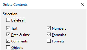
Data and cell formatting can be deleted from a cell at the same time. To do this:
1) Select a cell or a range of cells.
2) Press the Backspace key, or right-click in the cell selection and choose Clear Contents in the context menu, or select Sheet > Clear Cells on the Menu bar.
3) In the Delete Contents dialog (Figure 31), choose any of the options or Delete all.
4) Click OK.
Figure 31: Delete Contents dialog
To completely replace data in a cell and insert new data, select the cell and type in the new data. The new data will replace the old data but will retain the cell formatting.
Alternatively, select the cell and click in the Input line on the Formula bar (Figure 2 above), then double-click on the data to highlight it completely and type the new data.
Sometimes it is necessary to edit the contents of a cell without removing all of the data from the cell. For example, changing the phrase “Sales in Qtr. 2” to “Sales rose in Qtr” can be done as follows.
1) Click in the cell to select it.
2) Press F2 to switch the cell to edit mode. The cursor is placed at the end of the content in the cell.
3) Use the keyboard arrow keys to position the cursor where you want to start entering the new data in the cell, then press the Delete key or Backspace key to delete any unwanted data before typing the new data.
4) When you have finished editing, press the Enter key to save the changes.
Tip
You may want to enable Tools > Options > LibreOffice Calc > General > Press enter to switch to edit mode. Then, when you press the Enter key in a selected cell, the cell switches to edit mode, eliminating the need to press F2.
1) Double-click on the cell to select it and place the cursor in the cell for editing. You can also use Edit > Cell Edit Mode on the Menu bar to put the cell in edit mode.
2) Either:
Reposition the cursor to where you want to start entering the new data in the cell.
Single-click to select the cell, then move the cursor to the Input line on the Formula bar and click at the position where you want to start editing data in the cell.
3) When you have finished, click away from the cell to deselect it and save the changes.
To copy text, numbers, or formulas to the target cell or cell range:
1) Select the source cell or cell range and copy the data by pressing Ctrl+C or using Edit > Copy on the Menu bar.
2) Select the target cell or cell range.
3) Right-click on the target cell or cell range and select Paste Special in the context menu, then select Unformatted Text, Text, Number, or Formula.
Or, use the submenu items reached from Edit > Paste Special on the Menu bar.
You can also use the Paste Special function to paste into another cell selected parts of the data in the original cell or cell range, for example its format or the result of its formula. To do this:
1) Select a cell or a cell range.
2) Go to Edit > Copy on the Menu bar, or press Ctrl+C, or right-click and select Copy in the context menu.
3) Select the target cell or cell range.
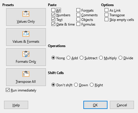
4) Go to Edit > Paste Special > Paste Special on the Menu bar, or use the keyboard shortcut Ctrl+Shift+V, or right-click and select Paste Special > Paste Special in the context menu to open the Paste Special dialog (Figure 32).
5) In the preset buttons on the left side of the dialog, you can choose to paste Values Only, Values & Formats, Formats Only, or to Transpose All the data in the target cells. On the right side of the dialog, select the options for Paste, Options, Operations, and Shift Cells. These are described in the Help and in Chapter 2, Entering, Editing, and Formatting Data, of the Calc Guide.
6) Click OK to paste the data into the target cell or range of cells and close the dialog.
Figure 32: Paste Special dialog
Tip
To see which combination of options on the right side would apply if one of the Preset buttons is selected, deselect the Run immediately option below the Presets. With the Run immediately option selected, clicking on a Preset button applies that combination of options and closes the dialog.
Note
All the settings discussed in this section can also be set as a part of the cell style. See Chapter 4, Using Styles and Templates, in the Calc Guide for more information.
Multiple lines of text can be entered into a single cell using automatic wrapping or manual line breaks. Each method is useful for different situations.
To automatically wrap multiple lines of text in a cell, use one of the following methods.
Method 1
1) Right-click on the cell and select Format Cells in the context menu to open the Format Cells dialog.
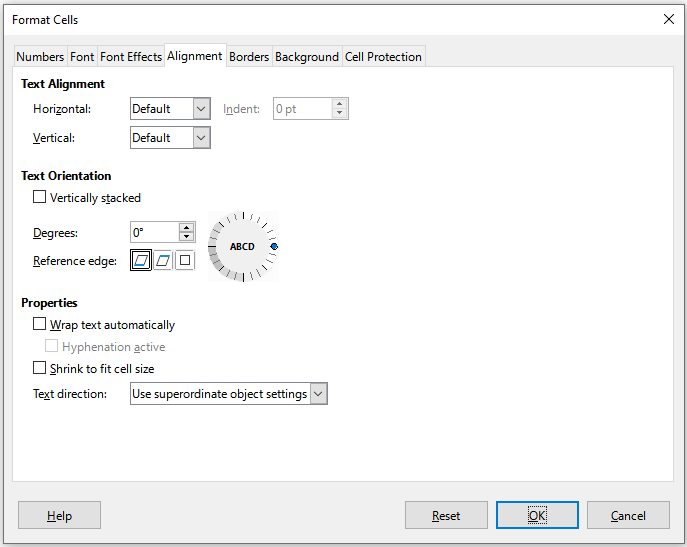
2) On the Alignment tab (Figure 33), under Properties, select Wrap text automatically and click OK.
Figure 33: Format Cells dialog – Alignment tab
Method 2
1) Select the cell.
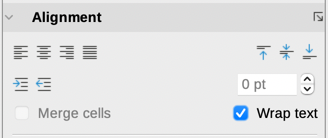
2) On the Properties deck of the Sidebar, open the Alignment panel (Figure 34).
3) Select the Wrap text option to apply the formatting immediately.
Figure 34: Wrap text formatting
To insert a manual line break while typing in a cell, press Ctrl+Enter. When editing text, double-click the cell, then reposition the cursor to where you want the line break. In the Input line of the Formula bar, you can also press Shift+Enter.
When a manual line break is entered in a cell, the cell row height changes but the cell width does not change and the text may still overlap the end of the cell. You have to change the cell width manually or reposition the line break.
The font size of the data in a cell can automatically adjust to fit inside cell borders. To do this, select the Shrink to fit cell size option under Properties on the Alignment tab of the Format Cells dialog (Figure 33).
You can select contiguous cells and merge them into one as follows:
1) Select the range of contiguous cells you want to merge.
2) Right-click on the selected cells and select Merge Cells in the context menu, or go to Format > Merge Cells > Merge Cells or Merge and Center Cells on the Menu bar, or click on the Merge and Center Cells icon on the Formatting toolbar. Using Merge and Center Cells will center align any contents in the cells.
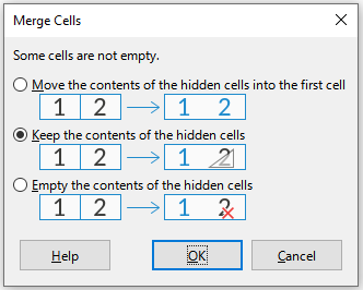
3) If the cells contain any data, a small dialog (Figure 35) opens, showing choices for moving or hiding data in the hidden cells. Make your selection and click OK.
Caution
Merging cells can lead to calculation errors in formulas used in the spreadsheet.
Figure 35: Merge choices for non-empty cells
You can split a cell that was created from several cells by merging.
1) Select a merged cell.
2) Go to Format > Merge Cells > Split Cells on the Menu bar, or right-click and select Split Cells in the context menu, or click on the Merge and Center Cells icon on the Formatting toolbar.
3) Any data in the cell will remain in the first cell. If the hidden cells did have any contents before the cells were merged, then you have to manually move the contents in to the correct cell.
Several number formats can be applied to cells by using icons on the Formatting toolbar. Select the cell, then click the relevant icon to change the number format.
For more control or to select other number formats, use the Numbers tab of the Format Cells dialog (Figure 25 above):
Apply any of the data types in the Category list to the data.
Control the number of decimal places and leading zeroes in the Options area.
Enter a custom format code.
The Language setting controls the local settings for the different formats such as the date format and currency symbol.
Some number formats are available on the sidebar’s Number Format panel of the Properties deck. Click the More Options button to open the Format Cells dialog.
Tip
For consistency in a spreadsheet, use cell styles whenever possible.
To manually select a font and format text for use in a cell:
1) Select a cell or cell range.
2) Click the small triangle on the right of the Font Name box on the Formatting toolbar and select a font in the drop-down list, or use the Font Name box in the Character panel of the Properties deck on the Sidebar.
3) Click on the small triangle on the right of the Font Size box on the Formatting toolbar and select a font size in the drop-down list, or use the Font Size box in the Character panel of the Properties deck on the Sidebar.
4) To change the character format, click on the Bold, Italic, or Underline icons on the Formatting toolbar or on the Character panel of the Properties deck of the Sidebar. On the Sidebar it is possible to change the underline appearance and add some extra effects to the font, such as Strikethrough and Shadow.
5) To change the horizontal paragraph alignment, click on one of the four alignment icons (Align Left, Align Center, Align Right, Justified) on the Formatting toolbar or on the Alignment panel of the Properties deck on the Sidebar. For more options, go to Format > Cells > Alignment and select one of the options in the Horizontal drop-down list.
6) To change the vertical alignment of the text in the cell, go to Format > Cells > Alignment and select one of the options in the Vertical drop-down list.
7) To change the font color, click the arrow next to the Font Color icon on the Formatting toolbar, or on the Character panel on the Properties deck of the Sidebar, to display the color palette, then select the desired color.
8) To specify the language used in the cell, use the Font tab on the Format Cells dialog.
9) Use the Font Effects tab on the Format Cells dialog to set other font characteristics.
To format the borders of a cell or a group of selected cells, click the Borders icon on the Formatting toolbar and select a border from the palette.
To format the border line style, click the Border Style icon on the Formatting toolbar and select the line style in the palette. For the color of the border lines, click the arrow at the right of the Border Color icon on the Formatting toolbar and choose from the selected color palette.
The Cell Appearance panel of the Properties deck on the Sidebar also contains cell border, line style and line color controls.
For more control, including the spacing between cell borders and any data in the cell, use the Borders tab of the Format Cells dialog, where you can also define a shadow style. Clicking the More Options button on the Cell Appearance panel, or clicking More Options in the panel’s line style drop-down list, opens the Format Cells dialog at the Borders tab.
See Chapter 4, Using Styles and Templates, in the Calc Guide for more information.
Note
Cell border properties apply only to the selected cells and can be changed only when you are editing those cells. For example, if cell C3 has a top border, that border can only be removed by selecting C3. It cannot be removed in C2 despite also appearing to be the bottom border for cell C2.
To format the background color for a cell or a group of cells, click the small arrow next to the Background Color icon on the Formatting toolbar. A color palette, similar to the Font Color palette, is displayed. You can also use the Background tab of the Format Cells dialog. The Cell Appearance panel of the Properties deck on the Sidebar contains a cell background control with a color palette. See Chapter 4, Using Styles and Templates, in the Calc Guide for more information.
To add default styles for a cell or a group of cells, click Styles on the Menu bar and a menu displays the default styles. The default styles can be applied, or modified in the Styles deck on the Sidebar. You can create custom cell styles by clicking Styles > New Style from Selection on the Menu bar, or by clicking the New Style from Selection icon on the Styles deck of the Sidebar, or by right-clicking a style in the Styles deck of the Sidebar and selecting New in the context menu. Type a new name for the style or click an existing style name to update that style. Apply, delete, or modify the custom style on the Styles deck.
You can use Calc’s AutoFormat feature to format a table (range of cells) quickly and easily. It also lets you format different tables of the sheet with the same look and feel very easily. All formatting applied is direct formatting.
1) Select the cells in at least three columns and rows, including column and row headers, that you want to format.
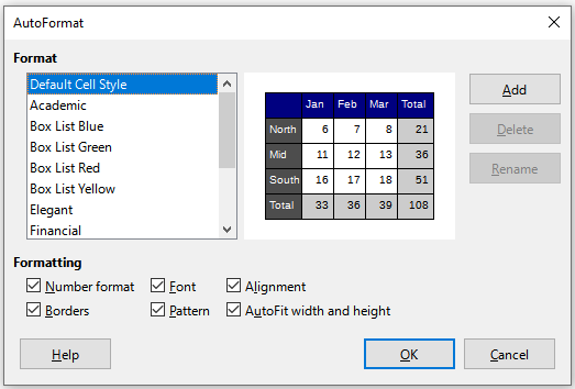
2) Go to Format > AutoFormat Styles on the Menu bar to open the AutoFormat dialog (Figure 36).
3) Select the type of format and format color in the list.
4) Select the formatting properties to be included in the AutoFormat style. Click OK.
Figure 36: AutoFormat dialog
You can define a new AutoFormat so that it becomes available for use in all spreadsheets.
1) Format the data type, font, font size, cell borders, cell background, and so on for a range of cells.
2) Select the range, of at least 4 x 4 cells.
3) Go to Format > AutoFormat Styles to open the AutoFormat dialog. Click Add.
4) In the Name box of the Add AutoFormat dialog that opens, type a meaningful name for the new format.
5) Click OK to save. The new AutoFormat is now available in the Format list in the AutoFormat dialog.
Note
The new AutoFormat is stored in your computer user profile and is not available to other users. However, other users can import the new AutoFormat by selecting the table range in the spreadsheet document and defining it as a new AutoFormat.
Calc comes with a predefined set of formatting themes (set of styles) that you can apply to spreadsheets. It is not possible to add new themes to Calc, but you can modify the theme styles after the theme is applied to the spreadsheet. The modified styles are available for use only in that spreadsheet.
To apply a theme to a spreadsheet:
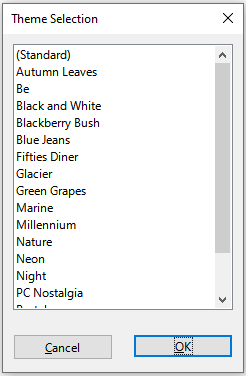
1) Go to Format > Spreadsheet Theme on the Menu bar or click the Spreadsheet Theme icon on the Tools toolbar to open the Theme Selection dialog (Figure 37).
2) Select the theme that you want to apply. The theme styles are immediately visible on the underlying spreadsheet.
3) Click OK.
6) If you wish, you can now open the Styles deck on the Sidebar to modify specific styles. These changes do not modify the theme; they only change the appearance of the style in the specific spreadsheet you are using. For more about modifying styles, see Chapter 3, Using Styles and Templates.
Caution
Applying a new theme over an existing one will override all existing theme styles customization with the new theme styles.
Figure 37: Theme Selection dialog
You can set up cell formats to change depending on conditions that you specify. For example, in a table of numbers, you can show all the values above the average in green and all those below the average in red. Multiple formatting options can be entered and arranged using assigned priority rules to order the importance of the conditions, allowing certain formatting options to take place before others.
Conditional formatting depends upon the use of styles, and the AutoCalculate feature (Data > Calculate > AutoCalculate) must be enabled. See Chapter 2, Entering, Editing, and Formatting Data, in the Calc Guide for details.
A filter is a list of conditions that each entry has to meet to be displayed. Calc provides three types of filter:
Setting up and using filters are explained in Chapter 2, Entering, Editing, and Formatting Data, of the Calc Guide.
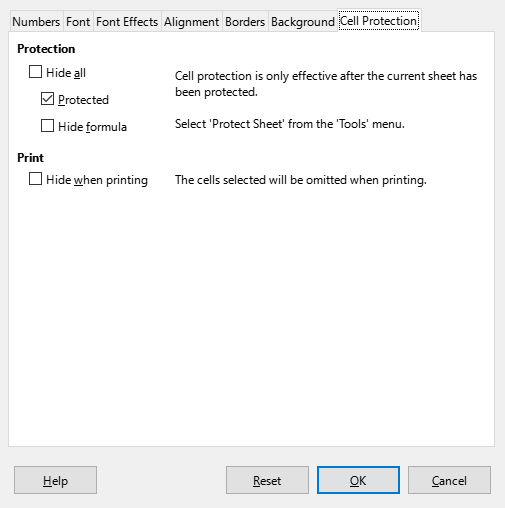
All or some of the cells in a spreadsheet can be password protected to prevent changes being made by unauthorized users. This can be useful when multiple people have access to the spreadsheet itself, but only a few are allowed to modify the data it contains. Protected cells can optionally be hidden.
Use the Cell Protection tab of the Format Cells dialog (Figure 38) to set up cell protection and toggle the hidden status of protected cells.
Figure 38: Cell Protection tab in Format Cells dialog
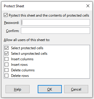
When all desired cells have been flagged with either a protected or unprotected status:
1) Go to Tools > Protect Sheet, or right-click on the sheet’s tab in the Sheet tabs area and select Protect Sheet in the context menu. The Protect Sheet dialog opens (Figure 39).
2) Select Protect this sheet and the contents of protected cells.
3) Type a password and then confirm the password.
4) Select or deselect the user selection options for cells.
5) Click OK.
Figure 39: Protect Sheet dialog
Any cells that had been toggled as protected will no longer be editable by anyone that does not have the password.
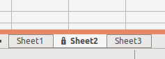
The protected sheet has a lock icon in its tab, as shown in Figure 40.
Figure 40: The lock icon in a protected sheet
Alternatively, you can protect the structure of the entire spreadsheet rather than individual cells on individual sheets by selecting Tools > Protect Spreadsheet Structure on the Menu bar. This option enables you to protect your spreadsheet against adding, deleting, moving, or renaming sheets. You can optionally enter a password on the Protect Spreadsheet Structure dialog.
Sorting within Calc arranges the cells in a sheet using the sort criteria that you specify. Several criteria can be used and a sort applies each criteria consecutively. Sorts are useful when you are searching for a particular item and become even more useful after you have filtered data.
Also, sorting is useful when you add new information to your spreadsheet. When a spreadsheet is long, it is usually easier to add new information at the bottom of the sheet, rather than adding rows in their correct place. After you have added information, you can then sort the records to update the spreadsheet.
For more information on how to sort records and the sorting options available, see Chapter 2, Entering, Editing, and Formatting Data, in the Calc Guide.
To sort cells in a spreadsheet using the Sort dialog:
1) Select the cells to be sorted.
2) Go to Data > Sort on the Menu bar, or click the Sort icon on the Standard toolbar, to open the Sort dialog (Figure 41).
Figure 41: Sort dialog, Sort Criteria tab
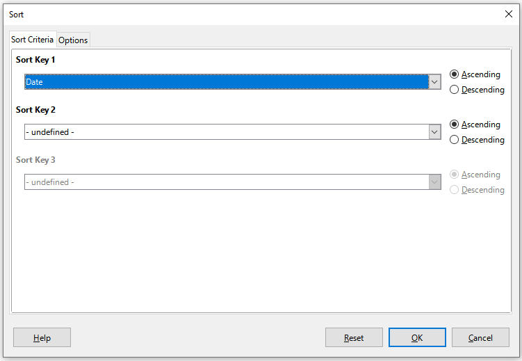
3) On the Sort Criteria tab, select the sort criteria in the drop-down lists. The selected lists are populated from the selected cells.
4) Select either ascending order (A-Z, 0-9) or descending order (Z-A, 9-0).
5) Adjust the settings as required on the Options tab. For details, see the Help or Chapter 2, Entering, Editing, and Formatting Data, of the Calc Guide.
6) Click OK and the sort is carried out on the spreadsheet.
Comments are small notes and text that can serve as a reminder or an aside to the user. A comment is not considered a part of the spreadsheet for calculation or printing purposes, and will only appear when hovering the mouse over the particular cell that has been commented.
The easiest way to insert a comment is by right-clicking on the desired cell and selecting Insert Comment in the context menu. Alternatively, you can select Insert > Comment on the Menu bar, or use Ctrl+Alt+C, or click the Insert Comment icon on the Standard toolbar.
By default, comments will remain hidden and only appear when hovering the mouse. Cells that contain comments are marked with a red square in the upper right corner. To toggle the visibility of comments, select View > Comments on the Menu bar.
For more information, see Chapter 11, Sharing and Reviewing Spreadsheets, in the Calc Guide.
You may need more than numbers and text in a spreadsheet. Often the contents of one cell depend on the contents of other cells. Formulas are equations that use numbers and variables to produce a result. Variables are placed in cells to hold data required by equations.
A function is a predefined calculation entered in a cell to help you analyze or manipulate data. All you have to do is enter the arguments and the calculation is made automatically. Functions help you create the formulas required to get the results that you are looking for.
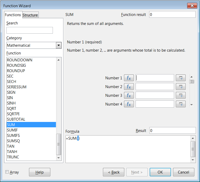
Functions and formulas can be entered directly into the Formula bar or by accessing the Function Wizard. To launch the function wizard, click the Function Wizard icon to the right of the Name Box, or select Insert > Function on the Menu bar, or press Ctrl+F2.
Inside the Function Wizard, you can search, list, and narrow down the many Calc functions available. You can also choose to complete functions from within the wizard rather than having to type full formulas into the Formula bar.
Each function, when selected, will display a brief explanation of its use and acceptable syntax. It will also display dialog boxes where you can enter the information required by that function and a result window showing the expected calculation from the data entered.
Note
A fast alternative to the Function Wizard is the Functions deck on the Sidebar, where you can quickly list and narrow down functions. It provides brief explanations on their use and syntax, but does not provide the search or data entry capabilities of the full wizard.
LibreOffice Calc offers powerful built-in functions under multiple domains or categories. They are: Database, Date & Time, Financial, Information, Logical, Mathematical, Array, Statistical, Spreadsheet, Text, and Add-in functions.
For a more in-depth introduction to formulas and the Function Wizard, see Chapter 7, Using Formulas and Functions, in the Calc Guide.
Figure 42: Function Wizard
Calc includes several tools to help you analyze the information in your spreadsheets, ranging from features for copying and reusing data, to creating subtotals automatically, to varying information to help you find the answers you need. These tools are divided between the Tools and Data menus.
Calc also includes many tools for statistical analysis of data, where you can obtain important numerical information on data obtained from physical measurements, polls, or even business transactions such as sales, stock quotations, and so on. These statistical data analyses are available in the menu Data > Statistics.
See Chapter 9, Data Analysis, in the Calc Guide for more information on the tools available.
One of the most useful tools for analyzing data is the pivot table, a way to organize, manipulate, and summarize large amounts of data to make it much easier to read and understand while also allowing you to answer different questions about a spreadsheet by rearranging – or pivoting – the data in it. Using a pivot table, you can view different summaries of the source data, display the details of areas of interest, and create reports. You can also create a pivot chart to view a graphical representation of the data in a pivot table.
For example, you might have a spreadsheet containing a list of donations to various charities by a group of recruiters in various months, but you are only interested in how much money each recruiter has collected in total. You could manually calculate that amount by using the sorting and formatting options provided by Calc. Alternatively, you could arrange a pivot table to make that data easier to organize and read.
To create a pivot table, choose Data > Pivot Table > Insert or Edit on the Menu bar, or click the Insert or Edit Pivot Table icon on the Standard toolbar. The Pivot Table Layout dialog will intelligently guess the column headings from the provided raw data and insert them into the Available Fields selection box. From there, you can drag and drop your desired information into column, row, data, or filter fields to organize accordingly and click OK to view the results.
To choose new information to display, or to alter the layout of the existing information, right-click anywhere in the existing pivot table to bring up the context menu and choose Properties. You can also access the same dialog by selecting Data > Pivot Table > Insert or Edit on the Menu bar, or clicking the Insert or Edit Pivot Table icon on the Standard toolbar.
For an in-depth explanation of pivot tables and the preconditions necessary to use them, see Chapter 8, Using Pivot Tables, in the Calc Guide.
To get a quick visual representation of the data contained in a pivot table, you can generate a pivot chart. Functionally, pivot charts are nearly identical to regular charts except in two key areas. First, as the data in the pivot table is altered, the pivot chart will adjust itself automatically. Second, it includes field buttons, graphical elements that allow you to filter the content of the pivot table from within the pivot chart itself.
For more information on pivot charts and charts in general, see Chapter 3, Creating Charts and Graphs, and Chapter 8, Using Pivot Tables, in the Calc Guide.
Printing from Calc is much the same as printing from other LibreOffice components (see Chapter 10, Printing, Exporting, E-mailing, and Signing Documents). However, some details of printing in Calc are different, especially regarding preparation for printing.
After print ranges have been defined, they are formatted with automatic page breaks. To view the page breaks, go to View > Page Break on the Menu bar.
Print ranges have several uses, including printing only a specific part of the data or printing selected rows or columns on every page. For more information about using print ranges, see Chapter 6, Printing, Exporting, Emailing, and Signing in the Calc Guide.
To define a new print range or modify an existing print range:
1) Select the range of cells to be included in the print range.
2) Go to Format > Print Ranges > Define on the Menu bar. Automatic page break lines are displayed on screen.
3) To check the print range, go to File > Print Preview on the Menu bar, press Ctrl+Shift+O, or click the Toggle Print Preview icon on the Standard toolbar. Calc will display only the cells in the print range.
After defining a print range, you can add more cells to it by creating another print range. This allows multiple, separate areas of the same sheet to be printed while not printing the whole sheet.
1) After defining a print range, select an extra range of cells for adding to the print range.
2) Go to Format > Print Ranges > Add on the Menu bar to add the extra cells to the print range. The page break lines are no longer displayed on the screen.
3) To check the print ranges, go to File > Print Preview on the Menu bar, press Ctrl+Shift+O, or click the Toggle Print Preview icon on the Standard toolbar. LibreOffice will display the print ranges as separate pages.
Note
The additional print range will print as a separate page, even if both ranges are on the same sheet.
It may become necessary to remove a defined print range, for example, if the whole sheet needs to be printed later.
To remove all the defined print ranges, go to Format > Print Ranges > Clear on the Menu bar. After the print ranges have been removed, the default page break lines will appear on the screen.
At any time, you can directly edit the print range, for example to remove or resize part of the print range. Go to Format > Print Ranges > Edit on the Menu bar to open the Edit Print Ranges dialog where you can define the print range.
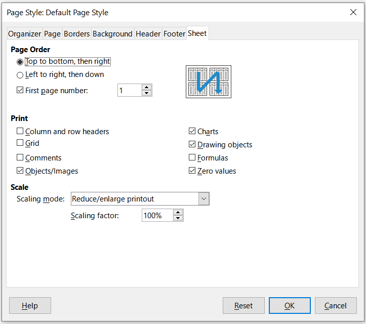
To select the printing options for page order, details, and scale to be used when printing a spreadsheet:
1) Go to Format > Page Style on the Menu bar to open the Page Style dialog (Figure 43).
2) Select the Sheet tab and make your selections from the available options. Click OK.
Figure 43: Page Style dialog – Sheet tab
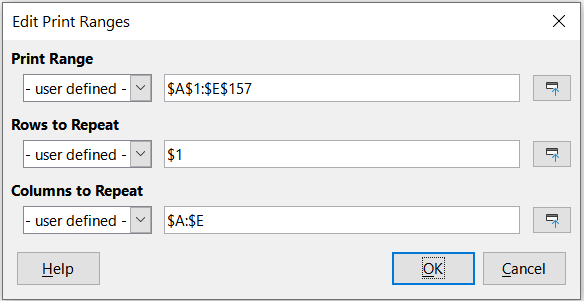
If a sheet is printed on multiple pages, you can set up certain rows or columns to repeat on each printed page. For example, if the top two rows of the sheet as well as column A need to be printed on all pages, do the following:
1) Go to Format > Print Ranges > Edit on the Menu bar to open the Edit Print Ranges dialog (Figure 44).
2) Type the row identifiers in the Rows to Repeat box. For example, to repeat rows 1 and 2, type $1:$2. This automatically changes Rows to Repeat from - none - to - user defined -.
3) Type the column identifiers in the Columns to Repeat box. For example, to repeat column A, type $A. In the Columns to Repeat list, - none - changes to - user defined -.
4) Click OK.
For more information on editing print ranges, see Chapter 6, Printing, Exporting, E-mailing, and Signing, in the Calc Guide.
Figure 44: Edit Print Ranges dialog
While defining a print range can be a powerful tool, it may sometimes be necessary to manually adjust the Calc printout manually using a manual or page break. A page break helps to ensure that the data prints properly according to the page size and page orientation. You can insert a horizontal page break above or a vertical page break to the left of the active cell.
To insert a page break:
1) Navigate to the cell where the page break will begin.
2) Go to Sheet > Insert Page Break on the Menu bar.
3) Select Row Break to create a page break above the selected cell. Select Column Break to create a page break to the left of the selected cell.
To remove a page break:
1) Navigate to a cell that is next to the break you want to remove.
2) Go to Sheet > Delete Page Break on the Menu bar.
3) Select Row Break or Column Break as needed.
Note
Multiple manual row and column breaks can exist on the same page. When you want to remove them, you have to remove each break individually.
For more information on manual breaks, see Chapter 6, Printing, Exporting, E-mailing, and Signing, in the Calc Guide.
Headers and footers are predefined pieces of text that are printed at the top or bottom of a page when a spreadsheet is printed. Headers and footers are set and defined using the same method. For more information on setting and defining headers and footers, see Chapter 6, Printing, Exporting, E-mailing, and Signing, in the Calc Guide.
Headers and footers are also assigned to a page style. You can define more than one page style for a spreadsheet and assign different page styles to different sheets within a spreadsheet. For more information, see Chapter 4, Using Styles and Templates, in the Calc Guide.
To set a header or footer:
1) Select the sheet that you want to set the header or footer for.
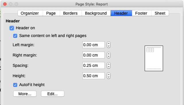
2) Go to Format > Page Style on the Menu bar to open the Page Style dialog (Figure 45) and select the Header or Footer tab (Figure 45).
3) Select the Header on or Footer on option.
4) Select Same content on left and right pages if you want the same header or footer to appear on all the printed pages.
5) Set the margins, spacing, and height for the header or footer. You can also select AutoFit height to automatically adjust the height of the header or footer.
6) To change the appearance of the header or footer, click on More to open the Border / Background dialog.
7) To set the contents, for example page number, date and so on, that appear in the header or footer, click Edit to open the Header (or Footer) dialog.
Figure 45: Header tab of Page Style dialog